Assignment: Reaction Times#
Learning Outcomes#
Learning Goals
The goal of this module is to collect and analyse reaction times.
After completing this module, you will be able to: understand and describe reaction times explain the LATER model gather reaction time data plot reaction times on a reciprobit scale You write a brief report or present your findings
These learning outcomes correspond to the following course learning goals. At the end of this module, by focusing on reaction times, you will be able to:
describe psychophysical methods and analyse psychophysical data
describe and build elementary neural models
Optional Material
Some sections include dropdowns with background information or MATLAB code.
These are optional and not required for the exam.
Short in-text questions and exercises are required and may appear in the exam.
Data#
Downloads#
Download the Matlab files:
This contains for example the visual search experiment.
Research Data Management#
To keep your work organised and reproducible, set up a simple folder structure before you begin:
Create a main folder named NBP_reactiontime.
Inside this folder, create three subfolders:
data – for storing exported simulation data files
analysis – for your MATLAB scripts
figures – for saving plots and exported images
Place all MATLAB code in the analysis folder. Then create a new MATLAB script named data_analysis.m in this folder. You will use this script to run your simulations, analyse the output, and generate figures. Whenever your script produces data files or images, save them into the corresponding data or figures folder. This structure helps ensure your work is easy to navigate, reproducible, and ready for future assignments. For additional guidance, see Research Data Management.
Background#
Reaction times are weird: they are slow, are stochastic and their distribution is not a standard one. Still, reaction times are measured extensively by psychophysicists and neuroscientists to study:
perception
attention
decision making
motor control
The previous module (Reaction Times) tried to give you an understanding of why reaction times are so interesting, and this module will delve deeper by exposing you to real reaction time experiments. We will see that the weirdness of reaction times are a feature, that might underlie optimal decision making in an uncertain world. In this module, you will analyse self-generated reaction times.
Scope of this module#
During the application session, you will record your own reaction time data for a visual search and an auditory detection paradigm. You will analyze this data by creating reciprobit plots.
1. Visual Search Experiment#
Background#
A central question in perception and systems neuroscience is how the brain parses complex sensory scenes into meaningful elements. In vision, this process appears effortless: we immediately perceive objects in terms of color, orientation, shape, texture, and motion. Yet it is far from obvious which of these dimensions constitute fundamental building blocks—that is, features that are encoded early and efficiently by the visual system.
Neurophysiological studies often approach this question by searching for neurons tuned to particular stimulus properties. While informative, this strategy is inevitably influenced by the experimenter’s prior assumptions about which features matter. Behavioral psychology has therefore developed complementary approaches that infer feature representations directly from performance. One of the most influential examples is the visual search paradigm, introduced by [Treisman and Gelade, 1980].
In a visual search task, observers decide as quickly and accurately as possible whether a predefined target is present among a number of distractors. Crucially, reaction times are measured as a function of the number of items in the display (the set size). Two qualitatively different patterns are typically observed:
Feature (pop-out) search: If the target differs from distractors along a single salient dimension (for example, color), detection is fast and largely independent of set size.
Conjunction search: If the target is defined by a combination of features (for example, color and shape), reaction times tend to increase systematically as more distractors are added.
This difference has been interpreted as evidence that some features are processed in parallel across the visual field, whereas conjunctions require a more effortful, item-by-item evaluation. In many experiments, reaction times increase linearly with set size, and the slope is often steeper when the target is absent than when it is present — consistent with a self-terminating serial search, in which the process stops once the target is found.
Although visual search experiments are subject to many potential confounds (such as luminance differences, eye movements, spatial frequency content, and stimulus eccentricity), the overall pattern of results is remarkably robust. For this reason, the paradigm has played a major role in shaping theories of attention and perception. In this practical, we will replicate the core logic of this classic experiment and use it as a first introduction to reaction-time analysis.
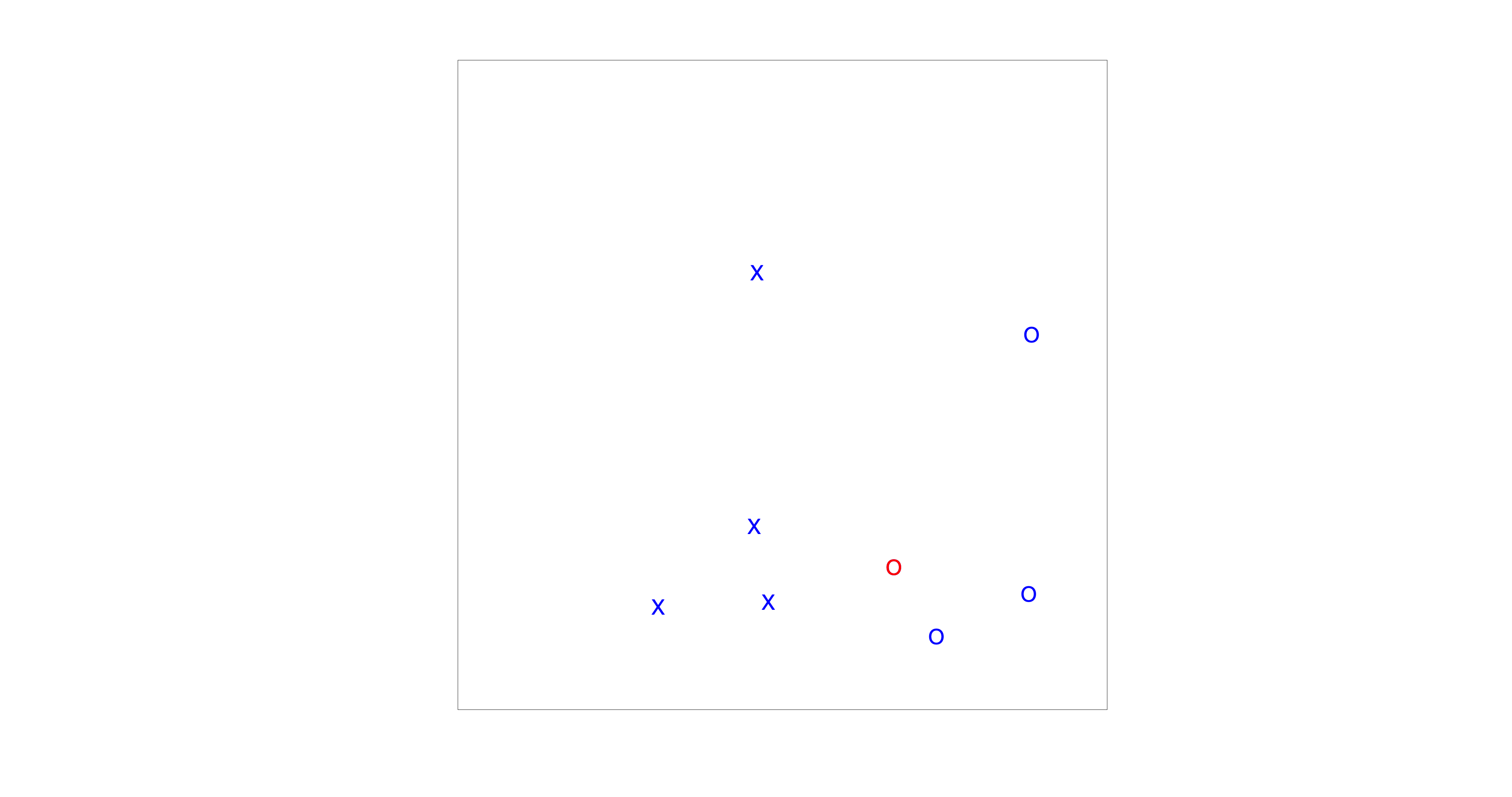
Fig. 85 The visual search paradigm used in this experiment.#
Experiment#
Reaction time distributions are a central theme of this course module, and visual search provides an intuitive and well-studied example. In this experiment (Fig. The visual search paradigm used in this experiment.), your task is to decide whether a red circle is present among a number of distractors.
Find the Red Circle
Go to your analysis folder and run visualsearchexp.m. You can start the experiment either from the editor or directly from the MATLAB command window:
visualsearchexp;
Choose your subject ID freely (this mainly matters if multiple people use the same computer).
On each trial, indicate whether the red circle is present or absent by pressing:
1 → target present
0 → target absent
Respond as quickly and accurately as possible.
Standard Analysis#
After completing the experiment, the data are automatically saved in the data directory. An example filename looks like:
visualsearch_sub-001_2025-12-17_15-28-05_seed-270243087.csv
This is a comma-separated values (CSV) file: a simple text format that can be opened in MATLAB, Excel, Numbers, or any text editor. The filename itself already contains useful metadata:
visualsearch – experiment name
sub-XXX – subject identifier
YYYY-MM-DD – date (chosen to allow chronological sorting)
HH-MM-SS – time of acquisition
seed-XXXX – random seed used to generate the stimulus order
To load your dataset into MATLAB, add the following lines to your data_analysis.m script:
fname = fullfile('..','data','visualsearch_sub-001_2025-12-17_15-28-05_seed-270243087.csv');
T = readtable(fname);
Make sure to replace the filename with the one corresponding to your experiment.
The data are stored in tidy format, meaning that each row corresponds to one trial and each column corresponds to a single variable. For example,
T(1,:)
displays the first trial. Important columns include:
rt – reaction time (in seconds)
targetPresent – whether the target was present (0 or 1)
setSize – number of items in the display (4, 8, 12, 16)
Csearch – search condition (pop-out vs conjunctive)
respKey – participant’s response (0 or 1; other values indicate invalid input)
Exercise: Analysing Visual Search Data
We will start with a standard analysis of visual search performance.
Consider only correct trials.
Plot median reaction time as a function of set size (4, 8, 12, 16).
Do this separately for the pop-out and conjunction conditions.
Compute overall accuracy.
Then answer the following questions:
Why is the median reaction time preferred over the mean?
Do your results qualitatively match the patterns described in the background?
How can you interpret the results in terms of classical reaction-time theory?
Why does reaction time depend on set size in conjunction search, but not (or much less) in pop-out search?
How would Donders explain a linear increase in reaction time with set size?
What might the intercept (fixed offset) of this linear relationship represent?
MATLAB Code
%% Exercise 1
% Read all data from a single directory

RT			= T.rt;
KP			= T.respKey;
Tpresent	= T.targetPresent;
N			= T.setSize;
C			= T.searchType;

% Only correct
sel		= KP==Tpresent ;
[sum(sel) sum(~sel) numel(sel) 100*sum(~sel)/numel(sel)] % some details on accuracy
RT		= RT(sel);
N		= N(sel);
C		= C(sel);

% First let's do a standard analysis, plotting median reaction times
X	= [C N];
Y	= RT;
[mu,ux] = assemble(Y,X,'fun',@median);

figure(1);
clf

sel = ux(:,1)==0;
x = ux(sel,2);
y = mu(sel);
h(1) = plot(x,y,'o-','MarkerFaceColor','w','LineWidth',2,'MarkerSize',12);
hold on
sel = ux(:,1)==1;
x = ux(sel,2);
y = mu(sel);
h(2) = plot(x,y,'s-','MarkerFaceColor','w','LineWidth',2,'MarkerSize',12);
nicegraph;

set(gca,'XTick',unique(X));
xlabel('set size');
ylabel('reaction time (ms)');

xlim([3 17]);

legend(h,{'pop-out','conjunctive'},'Location','NW');


% optional, save figure
fname = fullfile('..','..','images',[mfilename '_standard_ori.svg']);
savegraph(fname,'svg');
Distribution#
Next, we examine the shape of the reaction time distribution and test whether it is consistent with predictions from the LATER model (Reaction Times). Empirically, reaction times are rarely symmetrically distributed. Instead, they typically show a right-skewed distribution, with a long tail of slower responses.
The LATER model provides a simple explanation for this skewness. It assumes that decisions are triggered when a decision signal reaches a fixed threshold, and that the rate of rise of this signal varies randomly from trial to trial. If this rate is normally distributed, then reaction times themselves will be skewed, but their reciprocal—called promptness \(\frac{1}{RT}\) —should follow a Gaussian distribution.
Strictly speaking, the assumptions of the LATER model need not hold for visual search. Visual search, especially in the conjunctive condition, likely involves multiple perceptual and attentional stages (and possibly serial processing), whereas LATER describes a single stochastic accumulator. Nevertheless, visual search reaction time distributions are often qualitatively similar to those observed in simpler detection and discrimination tasks. In particular, when reaction times are transformed to promptness, the resulting distributions are frequently close to normal — provided that:
only correct trials are included,
anticipatory or accidental responses are excluded, and
the task involves a clear binary decision (target present vs absent).
In practice, our dataset contains too few trials per set size × search type condition to reliably assess distributional shape separately for each condition. However, for the pop-out condition, median reaction times do not depend on set size. This allows us to pool trials across set sizes without mixing distributions with different means.
Such pooling would not be appropriate for the conjunction search, where reaction times systematically increase with set size. Pooling those trials would combine distributions with very different means, resulting in a broad or even multimodal distribution that cannot meaningfully be compared to a normal distribution.
Exercise: Reaction Time Stochasticity
We will now analyse the stochastic structure of reaction times in the visual search task.
Filter the data to include only correct trials, target-present trials, and pop-out search.
Plot histograms of:
reaction times
promptness \(\frac{1}{RT}\)
Perform a Lilliefors test to assess normality for both measures.
Then answer the following questions:
Are the reaction times normally distributed, or do you observe systematic deviations? Why would this be expected?
Does your visual inspection of the histograms agree with the outcome of the statistical test?
Is promptness closer to a normal distribution than reaction time?
To what extent do these results support the LATER model?
Are there responses (e.g. predictive, inattentive, or outlier responses) that should be excluded before interpreting the distributions?
What is the Lilliefors test?
The Lilliefors test is a statistical test used to assess whether data are compatible with a normal distribution when the mean and variance are estimated from the data itself.
It is a variant of the Kolmogorov–Smirnov test, adapted for realistic situations in which the parameters of the normal distribution are not known in advance.
Conceptually, the test works as follows:
First, a normal distribution is fitted to the data (using the sample mean and standard deviation).
The empirical cumulative distribution function (CDF) of the data is compared to the CDF of this fitted normal distribution.
The test statistic reflects the maximum deviation between the two CDFs.
A significant result indicates that the observed deviations are larger than expected under normality.
Important points to keep in mind:
With small sample sizes, the test has low power and may fail to detect deviations.
With large sample sizes, even tiny deviations may become significant.
Therefore, statistical tests of normality should always be interpreted alongside visual inspection (histograms, Q–Q plots, reciprobit plots).
In this practical, the Lilliefors test is used as a diagnostic tool, not as a definitive yes/no decision about the validity of the LATER model.
MATLAB Code
%% Exercise 2
% Extract variables from table

RT          = T.rt;
KP          = T.respKey;
Tpresent    = T.targetPresent;
N           = T.setSize;
C           = T.searchType;

% Select only correct trials, target present, pop-out search
sel = KP == Tpresent & Tpresent == 1 & C == 0;

[sum(sel) sum(~sel) numel(sel) 100*sum(~sel)/numel(sel)] % accuracy overview

RT = RT(sel);

figure(2); clf

% --- Reaction time distribution ---
subplot(1,2,1);
plotpost(RT,'xlim',[0 1.5],'showCurve',false);
xlabel('reaction time (s)');
ylabel('proportion of responses');
nicegraph;

h = lillietest(RT);
normalstr = {'data is normally distributed','data is not normally distributed'};
title(normalstr{double(h)+1});

% --- Promptness distribution ---
subplot(1,2,2);
Promptness = 1 ./ RT; % s^{-1}
plotpost(Promptness,'xlim',[0.5 3],'showCurve',false);
xlabel('promptness (s^{-1})');
ylabel('proportion');
nicegraph;

h = lillietest(Promptness);
title(normalstr{double(h)+1});

% optional: save figure
fname = fullfile('..','..','images',[mfilename '_promptness_ori.svg']);
savegraph(fname,'svg');
Reciprobit#
Next, we will visualise the reaction time distributions using a reciprobit plot. This plot combines two transformations:
The horizontal axis uses promptness \(1/\mathrm{RT}\) (hence “reci-”), which is the key variable in the LATER model.
The vertical axis shows the cumulative probability on a probit scale (hence “-probit”), which stretches the tails of the distribution.
Why do this? Because if a LATER-like decision process dominates (i.e., a fixed threshold and a normally distributed decision rate), then promptness should be approximately normally distributed, and the reciprobit plot should reveal this as a near straight line. Deviations from linearity (curvature, kinks, mixed slopes) are informative: they suggest mixtures of processes, outliers (anticipations / lapses), or departures from the single-accumulator assumption.
You can generate reciprobit plots with matlab/reactiontime/reciprobitplot.m (also included in the zip you downloaded). A more complete explanation is given in Reaction Times.
For the pop-out condition, median RT hardly changes with set size. That makes it difficult to see systematic changes in the distribution across conditions. In conjunction search, however, reaction times do change with set size, which lets us ask a sharper question:
As the task becomes harder (larger set size), do the reciprobit lines mainly shift, swivel, or rotate?
If the LATER model applies, these qualitative patterns map onto specific parameter changes (illustrated in Fig. 84):
Parallel shift (horizontal translation): consistent with a change in mean decision rate (faster/slower accumulation), with similar variability.
Swivel (fan around a common intercept region): consistent with a change in threshold (more/less cautious responding).
Rotation (change in slope): consistent with a change in rate variability (or added sources of variability), not just the mean rate.
In practice, visual search may involve multiple stages and may not follow strict LATER predictions—but the reciprobit plot is still a useful diagnostic of how distributions change with task difficulty.
What does “probit” mean?
In a reciprobit plot, the y-axis shows the cumulative probability (the CDF), but not on a linear 0–1 scale. Instead we use a probit scale, which is the inverse of the cumulative normal distribution:
where \(\Phi\) is the CDF of a standard normal distribution.
Intuitively:
On a linear probability axis, most of the interesting action is compressed near 0 and 1 (the tails).
The probit transform stretches those tails, so differences in rare fast and slow responses become easier to see.
If the underlying variable (here: promptness) is normally distributed, then its cumulative distribution becomes a straight line on a probit axis.
This is closely related to a Q–Q plot (which you may have seen in Statistics 1): both tools compare an empirical distribution to the normal distribution. A Q–Q plot compares quantiles directly; a reciprobit plot compares the CDF on a probability scale that makes normality appear linear.
So: straight reciprobit lines suggest “close to normal” promptness; curvature suggests deviations (mixtures, outliers, or additional processes).
Exercise: Reciprocity + Probit in one picture
We will now make reciprobit plots for the conjunction search condition.
Filter the data to include only correct trials and conjunction search.
Plot the reciprobit curves in one figure, using a different colour for each set size.
Then discuss:
How close are the reciprobit curves to straight lines (i.e., how compatible is promptness with normality)?
As set size increases, do the lines mostly shift, swivel, or rotate?
What would that imply in LATER terms (rate change, threshold change, variance change)?
How would you interpret this in terms of a visual search?
If the lines are not straight, what might be causing the deviations (mixtures of strategies, lapses, speed–accuracy trade-off, target-absent trials mixed in, etc.)?
MATLAB Code
%% Exercise 3 — Reciprocity plot for conjunction search

RT       = T.rt;
KP       = T.respKey;
Tpresent = T.targetPresent;
N        = T.setSize;
C        = T.searchType;

% Select only correct trials and conjunction search
sel = (KP == Tpresent) & (C == 1);

RT = RT(sel);
N  = N(sel);

uN = unique(N);
n  = numel(uN);

figure(3); clf; hold on

% x-axis in reciprobitplot is typically promptness (ms^-1 or s^-1 depending on function)
% choose a sensible range based on your RTs:
xl = sort(-1000 ./ [500 1000]);  % example limits used in the original script

col = lines(n);
h = gobjects(n,1);

for ii = 1:n
    selN = (N == uN(ii));
    [Y, XRECIP, STATS, h(ii)] = reciprobitplot( ...
        RT(selN), 'regress', true, 'Color', col(ii,:), 'xlim', xl);
end

legend(h, string(uN), 'Location', 'NW');
xlabel('promptness (1/RT)');
ylabel('cumulative probability (probit)');
nicegraph;
2. Sound Modulation Detection Experiment#
Background#
In this practical you will perform a reaction-time experiment in which you detect the onset of a modulation in sound. The paradigm is inspired by the ripple-detection experiments of Veugen et al. [Veugen et al., 2022].
Compared to the visual search task, this experiment is conceptually simpler but theoretically cleaner. The sound starts as spectrally flat noise and, after a variable delay, begins to modulate in time and frequency. These structured, moving patterns in the spectrogram are known as ripples.
Because the physical onset of the modulation is well defined, this task is particularly suitable for studying reaction-time distributions and interpreting them within the LATER framework. Throughout the analysis, the onset of the modulation is treated as the stimulus onset that triggers the decision process.
Experiment#
In this experiment your task is to detect any change in the sound.
Ripple Detection Task
Go to your analysis folder and run soundrippleexp.m. You can start the experiment either from the MATLAB editor or directly from the command window:
soundrippleexp;
Once started, the experiment runs continuously, without pauses between trials.
Choose your subject ID freely (this mainly matters if several students use the same computer).
On each trial, press a key as soon as you perceive the modulation.
Respond as quickly and accurately as possible.
Analysis#
After the experiment finishes, the data are automatically saved in the data directory.
A typical filename looks like:
soundripple-subject-001-date-18-12-25-time-09-55-12.csv
This file is in comma-separated values (CSV) format, which can be opened in MATLAB, Excel, or any text editor.The filename itself already contains useful metadata:
soundripple – experiment name
subject-XXX – subject identifier
date-YYYY-MM-DD – acquisition date
time-HH-MM-SS – acquisition time
To load your dataset into MATLAB, add the following lines to your data_analysis.m script:
fname = fullfile('..','data','soundripple-subject-001-date-18-12-25-time-09-55-12.csv');
T = readtable(fname);
Replace the filename with the one corresponding to your own experiment.
The data are stored in tidy format: each row corresponds to one trial, and each column corresponds to a single variable.
Key variables include:
reactiontime – reaction time in seconds
velocity – temporal modulation rate (Hz)
density – spectral modulation density (cycles/octave)
Exercise: Analysing Ripple Detection Data
We begin with a standard analysis of ripple-detection performance.
Remove predictive responses and cap all late responses at 3 s.
Plot mean promptness as a function of
velocity (with density = 0)
density (with velocity = 0)
Visualise the spectrotemporal modulation transfer function (MTF) as an image.
Then answer the following questions:
Why is promptness preferred over reaction time in this analysis?
Do your results qualitatively match the patterns reported in [Veugen et al., 2022]?
How can you interpret these results in terms of classical reaction-time theory?
Why should reaction time depend on modulation velocity and density?
MATLAB Code
%% Exercise 1
% Read all data from a single directory

RT			= T.reactiontime;
v			= T.velocity;
d			= T.density;
durstat		= T.durstat;
RT			= RT*1000-durstat;


% Not predictive
sel		= RT>100;
RT = RT(sel);
v = v(sel);
d = d(sel);

% Late responses
sel		= RT>2000;
RT(sel) = 3000;

% First let's do a standard analysis, plotting median reaction times
% only
sel = d==0;
x = v(sel);
y = RT(sel);

[mu,ux] = assemble(1000./y,x,'fun',@median);

figure(1);
clf
subplot(131)
plot(1:3,mu(2:4),'o-','MarkerFaceColor','w','LineWidth',2,'MarkerSize',12);
hold on
set(gca,'XTick',1:3,'XTickLabel',ux(2:4));
xlabel('velocity (Hz)');
ylabel('promptness (s^{-1})');
nicegraph;
xlim([0 4]);
% ylim([0 1])
% First let's do a standard analysis, plotting median reaction times
% only
sel = v==0;
x = d(sel);
y = RT(sel);

[mu,ux] = assemble(1000./y,x,'fun',@median);


subplot(132)
plot(1:3,mu(2:4),'o-','MarkerFaceColor','w','LineWidth',2,'MarkerSize',12);
hold on
set(gca,'XTick',1:3,'XTickLabel',ux(2:4));
xlabel('density (cyc/oct)');
ylabel('promptness (s^{-1})');

nicegraph;
xlim([0 4]);


% First let's do a standard analysis, plotting median reaction times
% only
x =[v d];
y = RT;

[mu,ux] = assemble(1000./y,x,'fun',@median);

mu = reshape(mu,4,4);
subplot(133)
imagesc(mu);
nicegraph;
xlabel('velocity');
ylabel('density');
set(gca,'XTick',1:4,'XTickLabel',unique(v),'YTick',1:4,'YTickLabel',unique(d))


% optional: save figure
fname = fullfile('..','..','figures',[mfilename '_standard_ori.svg']);
savegraph(fname, 'svg');
Reciprobit Plots#
Next, we examine the full reaction-time distributions using a reciprobit plot, which visualises promptness on a reciprocal-time axis against probit-scaled cumulative probability.
As the task becomes harder (i.e. modulations are more difficult to detect), do the reciprobit lines mainly shift, swivel, or rotate?
If the LATER model applies, these qualitative changes map onto specific parameter changes (see Fig. 84):
Parallel shift → change in mean decision rate
Swivel → change in decision threshold
Rotation → change in rate variability
Because ripple detection is a simple detection task with a clear stimulus onset, it is particularly well suited for this type of analysis.
Exercise: Reciprocity + Probit in One Figure
Create reciprobit plots for velocity and density separately.
Include only non-predictive trials and no joint spectrotemporal modulation.
Plot reciprobit curves in two subplots:
one for velocity
one for density Use a different colour for each modulation value.
Then discuss:
How straight are the reciprobit lines (i.e. how compatible is promptness with normality)?
As modulation difficulty increases, do the curves mainly shift, swivel, or rotate?
What does this imply in LATER terms (rate, threshold, or variability)?
If curves deviate from straight lines, what might explain this? (e.g. lapses, mixtures of strategies, speed–accuracy trade-offs)
There might be some outliers which you may need to remove to get nice plots. In the Matlab code below, you need to change the limits of normal RTs (now set to between 400 and 900 ms).
MATLAB Code
%% Exercise 2 Reciprobit plots
% Read all data from a single directory

RT			= T.reactiontime;
v			= T.velocity;
d			= T.density;
durstat		= T.durstat;
RT			= RT*1000-durstat;

% Not predictive
sel		= RT>100;
RT = RT(sel);
v = v(sel);
d = d(sel);

% Late responses
sel		= RT>2000;
RT(sel) = 3000;

uv = unique(v);
nv = numel(uv);

ud = unique(d);
nd = numel(ud);

col = lines(3);


figure(3);
clf
subplot(121)
hold on;
xl = sort(-1000./[300 1000]);
for ii = 2:nv
	% subplot(2,2,ii)
sel = v==uv(ii) & d==0 & RT>400 & RT<900;

[Y, XRECIP, STATS,h(ii)] = reciprobitplot(RT(sel),'regress',true,'Color',col(ii-1,:),'xlim',xl);
hold on;
end

subplot(122)
hold on;
xl = sort(-1000./[300 1000]);
for ii = 2:nd
	% subplot(2,2,ii)
sel = d==ud(ii) & v==0  & RT>400 & RT<900;
% sel = v==uv(ii) & d==0 & RT>400 & RT<900;

[Y, XRECIP, STATS,h(ii)] = reciprobitplot(RT(sel),'regress',true,'Color',col(ii-1,:),'xlim',xl);
hold on;
end