Assignment: Fourier decomposition#
Spectrum of a digital signal#
Background#
Fourier decomposition is the most common method to retrieve the frequency components of a signal. There are an infinite number ways of decomposing signals, and not all are useful, but Fourier analysis is. This decomposition method allows you to retrieve the frequencies of a signal, and you have seen examples of why that might be interesting for visual perception (spatial and temporal motion frequencies). For sound perception this kind of analysis is so important that even the sensory organ for hearing (the cochlea) analyzes incoming sounds in a Fourier-like fashion. In this assignment, you will analyse self-generated sounds.
Scope of this assignment#
You will generate a pure tone and record your own voice over Matlab in one of the computer rooms during the afternoon. You will analyze the frequency components of these signals. You will write a brief report during the computer practical (or afterwards).
Duration#
This assignment will take 2 to 4 hours, depending on your familiarity with Matlab.
Learning goals#
This assignment has been developed to support you to achieve the following learning outcomes:
You decompose a digital signal in its frequency components
You analyze a signal with the Matlab implementation of the Fast Fourier Transform (FFT)
You plot basic figures using Matlab
You write a brief report
These learning outcomes correspond to the following course learning goals. At the end of this section, you will be able to:
analyse linear systems in the time domain and frequency domain, and
draw conclusions for the system’s response to arbitrary stimuli
Product#
You will make this assignment during the computer practical time allotted for this assignment (deadline a).
You will produce a brief report before next week’s practical (deadline b).
Instructions#
Generate and analyze sound signals. Just follow the description for this assignment.
Create a brief report. The report should contain all code and all figures made during the practical, with brief written explanation. The questions in this assignment should all be answered. The report should be a coherent story.
A pure tone#
First, we will generate and plot a pure tone (a pure tone is a sine wave):
x = 0:0.01:20;
y = sin(x);
plot(x,y);
The figure should look like Fig. Plotting a Sine Wave. This figure has small labels, no axis labels, no title, and no legend.. You may notice that the axis values are hard to read. This is easily solved:
set(gca,'FontSize',25);
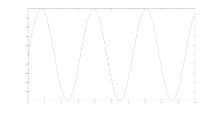
Fig. 7 Plotting a Sine Wave. This figure has small labels, no axis labels, no title, and no legend.#
question - sine wave frequency
What is the frequency of this sine wave if the x-axis would be time in sec?
Of course, this is not a relevant signal that we can hear as a pure tone. So, let’s make a pure-tone signal, plot it, and play it. Generate an array of 1000 elements, representing time from 0 to +100 msec, e.g. with the matlab routine linspace.
x = linspace(0,100,1000);
This time array has 1000 elements with a unit in msec. It is easier to have the unit in sec.
x = x/1000;
This is a digital signal, meaning that it consists of discrete elements or samples.
question - sampling frequency
What is the sampling frequency Fs of this signal (see also next section)?
We will make a pure tone with a frequency of 150 Hz.
f=150;
a phase of pi/6:
ph=pi/6;
and an amplitude of 1.5:
A=1.5;
question - sine parameters
What do these parameters mean? Briefly explain.
question - different frequencies
How does the pure tone frequency differ from its sampling frequency?
Generate the pure tone (call it y1 with the sin matlab routine).
help sin
We can plot the signal as shown above, with some slight modifications; we will plot the signal as a fat 'linewidth',2 red line 'r-'.
plot(x,y1,'r-','linewidth',2);
question - periodicity
How many peaks do you expect to see? Briefly explain.
You always need to provide the correct x-label and y-label and title texts to the figure (see below), and make the FontSize readable (see above).
xlabel('time (s)');

ylabel('amplitude (a.u.)');

title('150-Hz pure tone with phase pi/6 and amplitude 1.5');
You can play the signal over your speakers or headphones via the matlab-routine soundsc.
soundsc(y1,Fs);
Now, create a new pure tone (y2), with a frequency of 2000 Hz, a phase of pi/3 and amplitude 0.6, and plot this signal in the same figure hold on as a fat blue line (help plot, to find out what the letter code is for blue).
Also play this signal over your speakers or headphones via the matlab-routine soundsc.
question - perception
How would you describe the perceived difference? Which one is louder? Which one is higher-pitched? Which starts earlier?
Create a third signal (y3), summing both tones. Make a plot, in the same figure in black.
The amplitude spectrum#
Fast Fourier Transform#
We’re going to plot the spectrum of the first sine. This one’s a bit tricky! You will have learned about Fourier analysis for continuous, analog signals. We can also represent digital signals in the frequency domain, but this requires a computer algorithm that can theoretically and pragmatically do this: the world-wide known routine called ‘Fast Fourier Transform’, or FFT. To use this routine correctly, however, we will have to use some important tricks, so pay attention!
First, the routine needs a number of input points, which is a power of two (i.e. 2, 4, 8, 16, 32, 64, 128, 256, 512, 1024, 2048, 4096, etc.). So, if your signal has, say 1000 points, you should tell the routine to expand it to 1024 (it does so by simply adding zeros). Note, however, that we should also pay attention to the fact that the signal should ‘start and end smoothly’ in zero! For this simple example, we will not do that, but later, when we generate tones, we will carefully incorporate this ‘smoothness’ demand! So invoke the following command (suppose your 150 Hz sine wave is stored in array y1):
ft=fft(y1, 1024);
You now have created the spectral representation of the sine wave, but this is made of 1024 (using \mcode{whos}) complex numbers (you can see this by showing the first 5 entries on your computer):
whos ft

ft(1:5)
This basically doubles the amount of information since a complex number consists of both a real and an imaginary number. However, according to the mathematics, only half of this array contains the relevant frequency information. We therefore only take the first 512 numbers
ft=ft(1:512);
The reason is, that the original 1024 numbers contain both the amplitudes of the spectrum and the phases of the sines at each frequency of the spectrum.
question - mirror
Briefly explain in your own words why you only need to keep half of the FFT signal.
Amplitude characteristic#
Next, we determine the magnitude of the spectrum by taking the absolute values of the 512 complex numbers:
fa = abs(ft);
So now we have real-valued numbers again. Finally, we have to think about the frequency scale. We have 512 numbers, and they represent frequency, but how? This, of course, is determined by our original time axis! The time runs from -10 ms to +90 ms in 1000 samples, which means that the sampling interval \(\Delta T = 0.1/1000=0.0001\) s. The maximum frequency corresponding to this minimum interval is then \(1/\Delta T=10\) kHz. The Fourier algorithm fft then represents the spectrum to exactly half of this maximum frequency (see above), which is 5000 Hz. So now we know that our 512 frequency samples run from 0 to 5000 Hz. Thus, we can generate a frequency axis, say freq, just like the time axis above, with linspace. If you then plot fa against freq, you will see it nicely peak at the correct frequency.
question - correct frequency
Verify this!
question - log-scale
Apply the Matlab fft routine to determine the spectral content of the other signals. Make a plot of their spectrum on a log-frequency scale (the plot-routine you use is then semilogx).
Verify that the signal frequencies are correct!
You may notice that the amplitude (y-axis value) in the spectrum does not seem to correspond to the amplitude that you used for generating the pure-tone waveform. While it goes beyond this course to discuss why that is, note that you can get a better (not perfect) amplitude estimate of the spectrum by dividing by the length of the signal (each sample adds to the spectrum amplitude, so you have to normalize by the number of samples in a signal) and multiplying by 2 (because you threw away half of the data).
question - correct amplitude
For your brief report, only plot the correctly processed amplitudes.
The spectrogram#
We will extend Fourier analysis as applied to stationary signals to also cover nonstationary, dynamic signals. Pure tones are signals that never change (at least theoretically, or for the time period of interest). More interesting signals, such as speech and music, however, do change (this statement not only holds for acoustic signals). Fourier analysis assumes that the signals are stationary and periodic (i.e. the signals repeat). How can we use the Fourier transform to a nonstationary signal? By determining the Fourier spectrum over small intervals (short time windows) of the signal. Matlab’s signal processing toolbox provides the function spectrogram, which calculates a short-time Fourier transform (STFT).
You will first record a non-stationary signal, e.g. your own voice, which we can do with the function audiorecord. We will record only 1 channel (nchan) at a sampling frequency of 10 kHz (fs), the resolution of signal will be set at 16 bits (nbits),
r = audiorecorder(fs, nbits, nchan);
To start recording type:
record(r)
Now speak! (e.g. “we smell sausage”, or “the radio was playing too loudly”, http://auditoryneuroscience.com/elliott).
Once you have finished, you type:
stop(r)
You can play this back:
play(r)
And you can store it as a matrix:
mySpeech = getaudiodata(r);
Plot the temporal waveform of your signal (with readable and correct labels and units)!
Next, we will determine the STFT of this signal. Type:
spectrogram(mySpeech,256,'yaxis');
By default, spectrogram calculates the power of the signal into eight portions with overlap. The window size that we specified here was 256 samples, and we indicated that we wanted the y-axis to specify frequency (by providing the optional parameter ‘yaxis’). Since the sample frequency is not specified, the time scale will not be correct. To show the correct time and frequency scale, type:
spectrogram(mySpeech,256,[],[],fs,'yaxis');
question - spectrogram
Plot the spectrogram nicely. Briefly explain the spectrogram
What audio snippet did you use (what did you say)?
What do the colours mean?
When is the onset of speech in the signal?
Can you indicate word onset? Or can you indicate periods of silence?
Can you indicate examples of nonstationarity?
question - two-tone spectrogram
Plot the spectrogram of the two-tone signal (y3). Briefly explain.
Does that make sense?
Are the frequencies of the tones represented in the spectrogram?
Why can you see that this signal is stationary?
Follow-up#
In the application session (Application: Analyzing Voices) you will apply all knowledge to see how to analyze voice signals. In the module The Auditory System (The Auditory System), you will learn more about how sounds are processed in the brain, and you will see that the cochlea seems to process the frequencies of a sound in a Fourier-like fashion. In the modules on The Visual System, you will learn more about the visible spectrum of motion and depth perception.