Lab Assignment: Sound Localisation#
Learning Outcomes#
learning goals
This assignment has been developed to support you to achieve the following learning outcome:
You record your own sound localisation behavior
You can analyze your own sound localisation behavior
You write a brief report
At the end of this section, you will be able to:
Describe the three sound localisation cues (ITD/IPD, ILD/IID, spectral shape cues) accessible to humans and their features (binaural/interaural vs monaural, frequency range, horizontal/azimuth vs vertical/elevation localisation)
Explain the cone of confusion
Graph the (expected) stimulus-response plot for azimuth and elevation for broad-band, high-pass and low-pass noise stimuli
Explain the different results in the graphs in terms of availability (frequency range) and integration of cues (duplex theory)
Graph and explain the stimulus-response plot of a single-sided deaf individual (a monaural subject)
Describe the direction and frequency dependence of the binaural difference and the spectral cues of humans
Background#
Sound localisation plays an important role in directing attention to objects and events in our surrounding environment. This is not a trivial process, as the sensory cells for hearing are tuned to the frequency of a sound, and not its location. Sound localisation is possible because of the geometry of the head and the ears. This geometry yields binaural and monaural cues (see Lab Assignment: Head-Related Transfer Function) which our brains can process to determine sound source direction.
Scope of this assignment#
You will participate in a sound-localisation experiment (Fig. 20) in which you are asked to generate a rapid head movement toward a peripheral sound source (duration 150 ms), as soon as it appears. Three different sounds will be presented: broad-band noise (band width (BW) 0.2 – 20 kHz), low-pass filtered noise (BW: 0.2-1.5 kHz) and high-pass filtered noise (BW: 3.0-20 kHz). Stimuli also have different intensities, randomly varied between 40 and 70 dBA.
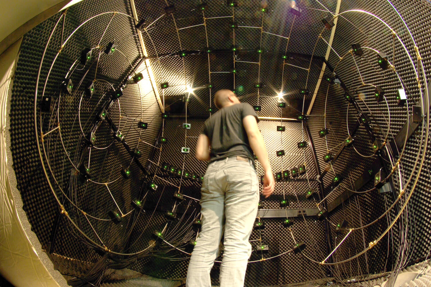
Fig. 20 Sound localisation setup. You will be seated in an anechoic room with 128 speakers positioned predominantly in the frontal hemisphere.#
After the experiments, your data collected will be returned to you (after pre-processing), and you will write a brief report on this.
Duration#
The experiment will take 20-30 min, and will typically be combined with the HRTF experiment (see Lab Assignment: Head-Related Transfer Function). Creating a report will take 2 to 4 hours, depending on your familiarity with Matlab.
Products#
You will have measured your sound localisation behavior before (deadline a).
You will produce a brief report (deadline b)
Criteria: The report should contain an Introduction, Methods, Results, and a Discussion, and it should be brief.
Instruction#
a. Sound localisation experiment
Register for a time-slot
Familiarise yourself with the methods and tools: knowledge clips 0n Brightspace.
Visit the lab and perform a sound-localisation experiment.
brief report
b. Create a brief report on the sound-localisation experiment
Produce a brief report of this measurement using the guidelines below. The report should contain a brief Introduction, Methods, Results, and a Discussion.
In the Introduction you should briefly describe the sound localisation cues, and predict how localisation behaviour is affected by a sound’s frequency content.
In the Methods, give a concise description of the stimuli (frequency content, locations), the task, and relevant information on the subject (i.e. you; e.g. the participant is a normal-hearing adult with no known visual or vestibular disorders that could affect the motor response).
In the Results, present your data in graphs (note: indicate variables!) of the stimulus-response relations for azimuth and elevation for each of the three stimulus types, and apply linear regression to quantify the results (see below for Matlab-related hints). Describe the results.
In the Discussion, explain the differences in (expected) results.
Data analysis and visualization#
Research Data Management#
All data collected in this experiment are stored on Brightspace. Each data file follows the naming convention:
XP-00ID-YY-MM-DD-BLCK
where:
XP – the experimenter’s initials
00ID – your personal 4-digit participant ID
YY – the 2-digit year when you performed the experiment
MM – the 2-digit month
DD – the 2-digit day
BLCK – the 4-digit experimental block number
For this assignment, you will organize your files in a clear directory structure on your local drive.
Create a main folder called NBP_sound.
Inside this folder, create three subfolders:
data
analysis
figures
Store your downloaded data files in the data folder. Then create a new MATLAB script named data_analysis.m and save it inside the analysis folder.
For more information, see Research Data Management.
Load data#
You need to load the data into Matlab’s workspace.
fname = fullfile('..','data','NB-0042-25-11-01.mat'); % this should be the file-name and path of your data set. Change this!
load(fname);
The data consists of a N x 8 matrix whose columns contain:
stimulus azimuth | stimulus elevation | stimulus frequency-band (1=BB, 2=HP, 3=LP) | stimulus level | response azimuth | response elevation | reaction time | participant id, and each row indicates trial number.
question - frequency bands
In the Introduction, explain:
the use of broadband, high-pass and low-pass sounds
how they relate to localisation cues
how well you expect those sounds to be localized
tidy data
The data is stored in tidy data format.
Stimulus-response plot#
You will visualise your sound localisation performance through a stimulus-response plot. A stimulus–response plot shows how a participant’s responses relate to the physical properties of the stimuli they were presented with. In this sound localisation experiment, each sound (stimulus) has a true position in space (in deg), and each response reflects where the listener thought the sound came from (also in deg). On the plot, the x-axis shows the stimulus location (the actual sound direction), and the y-axis shows the response location (the perceived direction). If responses are perfectly accurate, all points will fall on the diagonal (unity) line (i.e., response = stimulus). Deviations from the diagonal reveal biases (systematic shifts) or variability (scatter) in localisation performance. In short, a stimulus–response plot provides a simple visual summary of how precisely and accurately someone’s responses follow the presented stimuli.
Stimulus azimuth is presented in the first column, while response azimuth is encoded in the 5th column. You can make a stimulus-response plot, as follows:
stimaz      = Data(:,1); % stimulus azimuth in first column
resaz   = Data(:,5); % response azimuth in 5th column
plot(stimaz,resaz,'ko'); % plot responses as a function of azimuth
in which you explicitly extract the variables of interest (stimulus and response azimuth), and plot them.
Perfectly accurate and precise sound localisation responses should fall on the \(x=y\) (unity) line. Let’s modify the graph to visualize whether this also holds for your responses.
Note
Comments after the code lines (behind %) give a clue what that line is doing. Most of this is to have a nice figure, including plotting the \(x=y\) line and plotting open circles as symbols ko, but also automatically saving the figure.
 1stimaz      = Data(:,1); % stimulus azimuth in first column
 2resaz   = Data(:,5); % response azimuth in 5th column
 3
 4close all; % this will close all figures
 5figure(1); % this will open a figure and label it as 1
 6clf; % clear figure, in case this figure alreadt exists
 7plot(stimaz,resaz,'ko'); % plot responses as a function of azimuth
 8hold on; % if you want to plot
 9axis square; % make the figure square
10xlim([-95 95]); % limit the x-axis to run from -95 to +95 deg
11ylim([-95 95]); % limit the y-axis to run from -95 to +95 deg
12plot([-95 95],[-95 95],':'); % plot a dashed unity line ($x=y$)
13xlabel('stimulus azimuth (deg)'); % label the axes
14ylabel('response azimuth (deg)'); % label the axes
15title('sound azimuth localisation')
16figname = fullfile('..','figures','fig1.svg'); % the filename and relative path in which your figures are stored
17saveas(gcf, figname, 'svg'); % save the figure
Selection#
You will now have plotted all responses to all stimuli, but you are interested in whether the various sound frequency-bands elicit different responses. You can select the data by using a selection vector.
selection vector
A selection vector is a way to choose specific parts of your data in MATLAB. It is a logical vector (made of 1s and 0s or true/false values) that tells MATLAB which data points to keep. For example, suppose you have a vector of stimulus angles stim and you only want the trials where the sound was on the left (negative angles), in stim_left. You can create a selection vector sel like this:
stim    = [-30, -15, 0, 15, 30];
sel     = stim < 0;
stim_left = stim(sel);
This gives: sel = [1 1 0 0 0] and this is used to select only those elements in the last line, giving stim_left = [-30, -15] (i.e. only those values where the selection vector is 1 or true). So, a selection vector helps you extract the subset of data you need, for example, only correct trials, only left-side sounds, or only a particular condition, before making your stimulus–response plot.
For the sound-localisation data set, you are interested in the frequency-band, which is stored in column 3. To select for broadband noises you create a selection vector by finding all data equal to 1 (=the index for broadband sounds):
freq        = Data(:,3); % the frequency band is stored in column 3
sel         = freq==1; % selection vector, here selecting all frequencies freq equal to 1, which is the broadband sound
stimaz      = Data(sel,1); % stimulus azimuth in first column
resaz 	    = Data(sel,5); % response azimuth in 5th column
subplot(2,3,1); % create a 6 plots in the figure, in 2 rows and 3 columns, and making the first plot (top-left) active
plot(stimaz,resaz,'ko'); \% plot responses as a function of azimuth
Note
The selection vector contains only 0s (when the sound is not broadband) and 1s (when the sound is broadband). By using this selection vector, Matlab will keep only those values where the selection vector is 1 and remove those where the selection vector is 0. Note that you also used a subplot, to graph the stimulus-response plot in the upper left corner of the figure.
Statistics: linear regression#
Next up, you will quantify the stimulus-response relationship through linear regression. One way doing this is via:
1B       = regstats(resaz,stimaz,'linear'); % do linear regression
2slope   = B.beta(2); % the slope of the line
3offset  = B.beta(1); % the offset of the line
4xpred   = [-90 90]; % we will predict the response to these stimulus locations
5ypred   = offset+slope.*[-90 90]; % the response prediction
6plot(xpred,ypred,'r-','LineWidth',2); % and we plot the best-fit regression line, as a thick red line
This code extracts lots of parameters (B, line 1) related to linear regression, including the slope (line 2) and the offset (line 3). For now, you will only deal with the slope and the offset:
question - linearity
The auditory system clearly is a non-linear system. Is the stimulus-response relation for sound localisation linear?
in Methods, describe data and statistical analysis methods in Methods i.e., e.g. “using Matlab, we perform linear regression: y=ax+b, with x stimulus (deg), y response (deg), a gain with 1 indicating perfect accuracy…”.
In Results, describe how well the sound is localised
For-loops: other sounds#
You have now analysed and visualised the broadband sound localisation response. You will repeat these steps to plot and fit the stimulus-response relationships for azimuth and elevation and all three frequency bands. Whenever you have to repeat something, you can use a for-loop. A for-loop in MATLAB lets you repeat a set of commands several times, for example, once for each block, participant, or stimulus. It automatically steps through a list of numbers or items, running the same code for each step.
Basic example:
for i = 1:5
    i
end
This loop repeats the command inside five times, with i taking the values 1, 2, 3, 4, 5. You can use a for-loop to:
Load and analyse data from several blocks or participants
Compute results for different stimulus conditions
Create multiple plots in sequence
In your sound-localisation experiment, you might use a for-loop to make a stimulus–response plot for each stimulus, without having to copy-paste your code many times. Since you have three sounds, your code might look like this:
for ii = 1:3 % I typically use ii instead of i to prevent confusion with an imaginary number
    sel = freq==ii; % select frequencies equal to 1, then 2, then 3
    x = Data(sel,1); % determine the horizontal stimulus location
    y = Data(sel,5); % determine the vertical stimulus location
    subplot(1,3,ii); % plot in the first subplot, then second, then third
    plot(x,y,'.'); % actual plotting

end
You could also make it more robust, and not hard-code the frequencies (line 1 and 2). In the same for-loop, you could both plot (lines 18-20, 29-31) and do linear regression (lines 15-17, 26-28). You could also give titles to each column (lines 3, 21).
 1ufreq = unique(freq); % the unique frequencies, will be [1, 2, 3]
 2nfreq = numel(ufreq);
 3titletxt = {'broadband','highpass','lowpass'}; % this is a cell array of strings
 4
 5figure(2)
 6clf
 7slope = zeros(nfreq,2); % you have to initialise a matrix
 8offset = zeros(nfreq,2);
 9for ii = 1:nfreq
10    sel = freq==ufreq(ii); % select current frequency
11
12    % Azimuth
13    x = Data(sel,1); % determine the horizontal stimulus location
14    y = Data(sel,5); % determine the vertical stimulus location
15    B = regstats(y,x,'linear');
16    slope(ii,1) = B.beta(2);
17    offset(ii,1) = B.beta(1);
18    subplot(2,3,ii); % plot in the first subplot, then second, then third
19    plot(x,y,'.'); % actual plotting
20    hold on
21    title(titletxt{ii});
22
23    % Elevation
24    x = Data(sel,2); % determine the horizontal stimulus location
25    y = Data(sel,6); % determine the vertical stimulus location
26    B = regstats(y,x,'linear');
27    slope(ii,2) = B.beta(2);
28    offset(ii,2) = B.beta(1);
29    subplot(2,3,ii+3); % plot in the first subplot, then second, then third
30    plot(x,y,'.'); % actual plotting
31    hold on
32
33end
You yourself will need to visualise the data in a nice format, put labels on the axes, plot the regression lines, save the figure, as done before.
question - slopes and offsets
Determine the slopes and offsets for azimuth and elevation and all three frequency bands, and put them in a table. Also, plot the best-fit regression as a bold, red line in the subplots.
question - frequency band and localisation
In Results, describe how well each sound is localized for both horizontal and vertical directions.
For a Discussion, you can discuss:
the major findings
how your findings are in accordance with or in contrast to previous knowledge
why there are differences between sounds
whether the responses are as you expected
how the current experiment could provide more information and which other experimental manipulations might be useful in elucidating how human sound localisation works.
and explain briefly.
Note
So far, you have analysed only your sound localisation abilities. For an actual experiment, you would analyse these for all participants, and you would obtain summary statistics. You could do linear regression separately for each participant, determine the best-fit slope and offset, and then estimate or test (e.g. ANOVA) whether the sounds yield different responses. You could also do Bayesian hierarchical linear regression.
Follow-up#
In the video clips and lectures of Module - Reaction Times, you will use this data to see how reaction times may differ between different stimuli. In the chapters on the saccadic system (The Saccadic System - Pulse-Step Generator,The Saccadic System - The Burst Generator, and The Saccadic System - Superior Colliculus) , you will learn more about how we can orient our gaze.