Signals

Brief overview

A “signal” refers to a physical or virtual representation of information. signals can vary with respect to time, space, or any other independent variable. Here are a few key points about signals:

• Representation of Information: signals carry information, such as audio signals carrying the variations in air pressure that represent sound, or electrical signals representing variations in voltage over time.

• Time-Dependency: Many signals are functions of time and are called time-domain signals. These can be continuous-time signals (analog) or discrete-time signals (digital).

• Mathematical Function: A signal can often be mathematically described as a function that maps an independent variable (like time) to a dependent variable (like amplitude).

• Types of signals: There are various types of signals, including deterministic (exactly definable mathematical functions) and random (described statistically due to unpredictability).

• signal Transformations: signals can be transformed from one form to another, such as from the time domain to the frequency domain, using tools like the Fourier Transform, to make analysis of certain characteristics easier.

• Systems Response: In systems theory, signals are inputs to systems, and the output signals are the system’s response. Studying how systems modify signals is a fundamental aspect of signals and systems.

In summary, signals are the fundamental entities in signals and systems theory that represent information, which can be analyzed, processed, and manipulated by systems to achieve various outcomes. In systems analysis, we will see there are some simple, elementary signals that allow us to fully characterize a system.

Signals

A time-varying signal can be represented as (x(t)). We will primarily focus on two signal classes — Periodic signals and Transient signals. A signal is a (bio)physical quantity, which (here) varies in a deterministic way (i.e., according to an explicit formula) with time. signals can be very complex, but there are only a few basic, elementary signals: the impulse, the step, the sinusoid, the complex exponential and white noise. All these signals are beautifully related in mathematical ways. We will focus mainly on the impulse and the sinusoid.

Definition

A signal is a description of how a variable changes as a function of another variable, typically time.

Signal properties

Signals can be classified based on two main criteria (Fig. 3): continuity (continuous or discrete) and periodicity (periodic or aperiodic/transient).

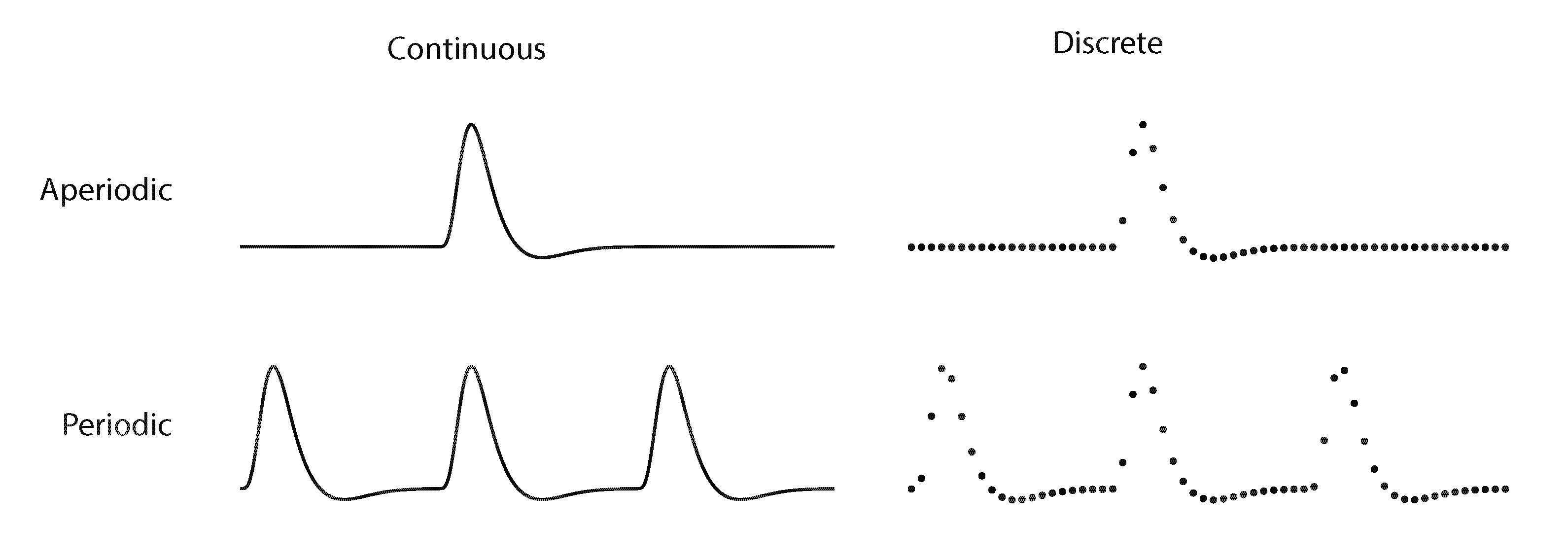
Fig. 3 illustration of the four types of signals.

Continuous vs. Discrete Signalss

• Continuous signals:

• Definition: A continuous signal is defined for every value of time and can take on any value. It’s represented as a smooth waveform.

• Examples in Neuroscience: Brain waves recorded by an EEG are typically seen as continuous signals.

• Characteristics: They have an infinite number of values within any given range and require analog processing techniques.

• Discrete signals:

• Definition: A discrete signal is defined only at specific time intervals and takes on discrete values. It’s often a result of sampling a continuous signal.

• Examples in Neuroscience: Spike counts in a given time interval or digitally sampled EEG data.

• Characteristics: They have a countable number of values and are suitable for digital processing.

Periodic vs. Aperiodic signals

• Periodic signals:

• Definition: A periodic signal repeats its pattern over a fixed, regular interval, known as the period.

• Examples in Neuroscience: Regular neuronal firing patterns or rhythmic brain waves like alpha rhythms in an EEG.

• Characteristics: They exhibit a repeatable pattern over time and are predictable after one period is observed.

• Aperiodic signals:

• Definition: An aperiodic signal does not repeat its pattern over regular intervals. Its pattern may or may not be predictable but does not exhibit periodicity.

• Examples in Neuroscience: Irregular brain wave patterns during complex cognitive tasks or random neuronal firings.

• Characteristics: They are more complex to analyze as they don’t have a regular repeating pattern.

Decomposition

Introduction

In neuroscience, understanding how the brain processes information involves studying complex signals. These signals often consist of various components mixed together. Decomposition is a key concept used to analyze and understand these complex signals by breaking them down into two or more simpler parts. There are many ways to decompose a signal. For example, the number 42 can be decomposed in \(12+30\), \(6 \times 7\), \(52-10\), etc. Why would we want to do this? The goal of decomposition is to turn a complex problem into a simple one. For example, you have to multiply 4242 by 3. How would you do this? You could imagine 4242 sheep, triple this mental image, and start counting the imaginary sheep. More likely, you will decompose 4242 into thousands, hundreds, tens and units: \(4000+200+40+2\), multiply each of those components by 3, and sum: \(12000+600+120+6 =12726\).

Why Decomposition is Used in Neuroscience

• Simplifying Complex signals. The brain generates complex signals that are difficult to interpret directly. Decomposition breaks these signals down into simpler components, making it easier to analyze and understand the underlying processes.

• Identifying Specific Features. Different components of brain signals can represent distinct physiological or cognitive processes. Decomposition allows researchers to isolate and study these specific features in isolation. For example, different frequency bands in EEG (like alpha, beta, theta) are associated with different brain states and activities.

• Noise Reduction and Artifact Removal Real-world neural signals often contain noise and artifacts (unwanted signals not related to the brain activity of interest). Decomposition techniques can help separate these artifacts from the actual brain signals, thus improving the signal quality for analysis.

• Enhancing Data Analysis. Decomposition enables more efficient and effective data analysis. By reducing the complexity of the data, it allows for better application of statistical and machine learning tools, which might be less effective on the original, more complex data.

• Application in Diagnostics and Treatment. In clinical settings, decomposition of neural signals can aid in diagnosing neurological disorders (like epilepsy, where specific wave patterns are indicative of seizure activity) and in optimizing treatments (like deep brain stimulation, where specific signal components can guide the stimulation parameters).

Importantly, using simple signals can allow us to fully characterize a (linear) system! In this course, we will see how simple signals such as pulses, steps and sines allow us to determine the workings of the oculomotor, auditory and visual systems.

Types of Decomposition

There are several common types of decomposition. In this course, we will deal with the following:

• Impulse Decomposition: Refers to the process of breaking down a signal into a series of impulses (or delta functions) and their associated coefficients. This concept is rooted in the idea that many signals can be represented as a sum of scaled and shifted impulses.

• Fourier Decomposition: Breaks down a signal into sinusoids of different frequencies. This is useful for understanding the frequency content of neural signals.

• Step Decomposition; Similar to impulse decomposition, involves representing a signal in terms of a series of step functions. A step function, often denoted as \(u(t)\) (unit step function), is a function that is zero for all negative time and one for positive time, representing a sudden change or step in value.

• Singular Value Decomposition: A statistical method that reduces the dimensionality of the data, highlighting the most significant features.

Periodic signals

Periodic signals have a waveform that repeats over and over after a fixed time interval \(T_0\). This waveform does not necessarily have to be sinusoidal, but can be arbitrary! In mathematical notation, we write this as follows:

\[x(t) = x(t \pm n \cdot T_0 )\]

with \(T_0 = \) signal period, \(n\) an integer and \(f_0 = \frac{1}{T_0}=\) the fundamental or ground frequency of the signal.

The elementary periodic signal is the sinusoid or the harmonic function:

\[x(t) = A \cdot \sin{(2\pi \cdot f \cdot t + \phi)}\]

with \(f\) the frequency (in Hz), \(t\) is time (in s), \(\phi\) is the phase (when the sine starts), and \(A\) is the amplitude. This harmonic function has an infinite duration (it has always existed and will never end; or it starts at big bang, ends at big crunch). This function is also periodic (it repeats itself). If there are only 10 periods (e.g. it starts at time t = 0 s, and ends at t = 10 s), this is not a real sinusoid. It also never changes, therefore it does not carry any information.

We typically rewrite \(2\pi \cdot f\) as \(\omega\) as it is easier than always writing out \(2\pi \cdot f\):

\[x(t) = A \cdot \sin{(\omega \cdot t + \phi)}\]

with \(\omega\) being angular frequency (in radians).

Fourier Transform

Fourier

Each periodic signal can be written as a superposition (= addition) of harmonic (sinusoidal) signals, each of which has its own amplitude, frequency and phase.

Here the frequencies of the cosines are all integer multiples of the fundamental frequency of the periodic signal. This idea is so essential to the analysis of systems that we have to stop and think about it. In formula form:

If \(x(t) = x(t \pm n \cdot T_0 )\), with \(n \in Z\) then it is possible to write \(x(t)\) as:

(3)\[x(t) = \frac{a_0}{2} + \sum_{n=1}^{\infty} a_n \cos{(2 \pi \cdot n \cdot f_0 \cdot t)} + \sum_{n=1}^{\infty} b_n \sin{(2 \pi \cdot n \cdot f_0 \cdot t)}\]

Such a series is called a Fourier series and the numbers (\(a_n\), \(b_n\)) are the so-called Fourier coefficients. This set of coefficients is unique for each periodic signal. \(a_n\) are the amplitudes of the cosines in the sequence, and \(b_n\) are the amplitudes of the participating sines. According to Fourier, these coefficients can be calculated as follows for the periodic function \(x(t)\) (period \(T_0\)):

(4)\[a_n=\frac{2}{T_0}\int_{0}^{T_0} x(t) \cdot \cos{(2\pi \cdot n \cdot f_0 \cdot t)} dt \textrm{ and } b_n=\frac{2}{T_0}\int_{0}^{T_0} x(t) \cdot \sin{(2\pi \cdot n \cdot f_0 \cdot t)} dt\]

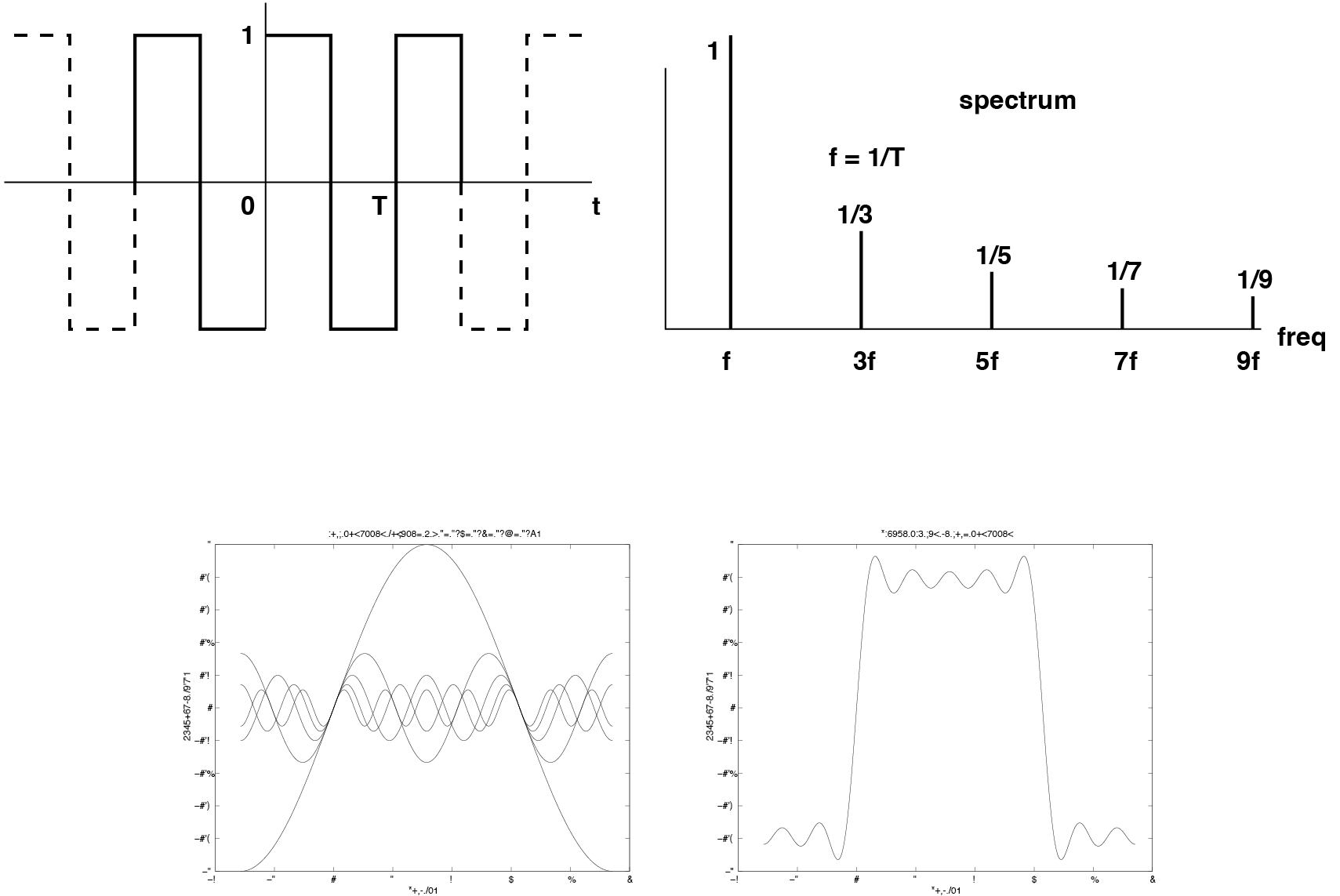
Fig. 4 Harmonic spectrum of a periodic square wave according to the Fourier series. B: Summation of the first five harmonic components comes quite close to a real square wave!

Now also note that if a periodic function is even (i.e. \(x(t) = x(-t)\) (symmetric with respect to the \(t = 0\) axis), that all \(b_n = 0\). If a periodic function is odd (that is, \(x(t) = -x(-t)\) (symmetric about the point \(t = 0\)), then all \(a_n = 0\). These symmetry properties can reduce the calculations of eqn_analysiseqn to half! In the next section (Exercises) we will try some simple examples on very simple periodic functions, such as the block function (see Fig. 4), to overcome the fear of using such formulas (and especially integrals). Take the following periodic function:

(5)\[x(t) = +1 \text{ for } 0 \leq t \leq 1 \textrm{ and } x(t) = -1 \text{ for } -1 \leq t < 0\]

and \(x(t)\) is periodic. Always ask yourself the following questions first:

• what is the period \(T_0\)

• is the function (coincidentally) even or odd?

• Then get started with Eqn. eqn_analysiseqn to calculate the Fourier coefficients!

• finally draw the spectrum (these are the Fourier coefficients) as a function of n.

In the exercises you will then also show that the following can be stated for trigonometric functions:

(6)\[a \cdot \cos{(x)} + b \cdot \sin{(x)} = c \cdot \cos{(x+\phi)}\]

(so the question becomes: how do \(c\) and \(\phi\) relate to \(a\) and \(b\).) The consequence of this trigonometric identity is that the Fourier series can also be written as (and that is how it is usually used):

(7)\[x(t) = \frac{a_0}{2} + \sum_{n=1}^{\infty} c_n \cos{(2 \pi \cdot n \cdot f_0 \cdot t + \phi_n)}\]

Here \(c_n\) are the amplitudes of the cosines in the series, \(\phi_n\) are the phases. Below are some examples of Fourier series. The entirety of different harmonic frequencies of the sinuses from which a signal according to this Fourier description is built up is called the spectrum of the signal (= frequency representation), and forms a complete representation of the signal properties in the same way as the time representation does. A signal therefore has different aspects:

• a time aspect.

• a frequency aspect (spectrum: cosines with their own amplitude and phase).

Note that the spectrum of a periodic signal has a large degree of regularity. All frequency components are integer multiples of the fundamental frequency. In other words: all frequencies are related to each other as rational fractions, or \(\frac{f_n}{f_m} \in Q\) for all \(n, m \in N\). Such a spectrum is a discrete spectrum (only certain frequencies are involved), and it is also harmonic. Figure Fig. 4 shows the periodic square wave. In addition, it can be seen how by adding sines of the correct amplitudes, frequencies and phases, the square wave can be approached more and more accurately. For this specific case it appears to apply (but you will show this neatly in the exercise section Exercises!):

\[x(t) \sim \sin{(2 \pi f_0 t)} + \frac{1}{3}\sin{(2 \pi (3 f_0) t)} + \frac{1}{5}\sin{(2 \pi (5 f_0) t)} + \frac{1}{7}\sin{(2 \pi (7 f_0) t)} + \dots\]

What we discussed here is the Fourier series, which holds for continuous and periodic signals. Each of the four signals (Fig. 3) has its own Fourier decomposition, three of which you only use when struggling with theoretical issues or doing homework (such as some of the exercises in this chapter). In practice, you will be using the Discrete Fourier Transform, which acts on discrete, periodic signals, because this is what computers can deal with. In chapter Assignment: Fourier decomposition, you will use a specific version of this, the Fast Fourier Transform.

Transient signals

Note that a periodic signal is assumed to live on an infinite time domain (\(-1 < t < +1\)). Such ideal signals do not occur in physical reality; usually a signal is defined from a certain starting moment (usually \(t = 0\)) up to some final moment (or not equal to 0). Such signals are called transient signals, and such signals also have a frequency spectrum. However, the associated spectra are no longer discrete (or harmonic), as for periodic signals, but continuous. This means that the number of frequency components in the spectrum are infinitely densely distributed (i.e. along one continuous frequency axis).

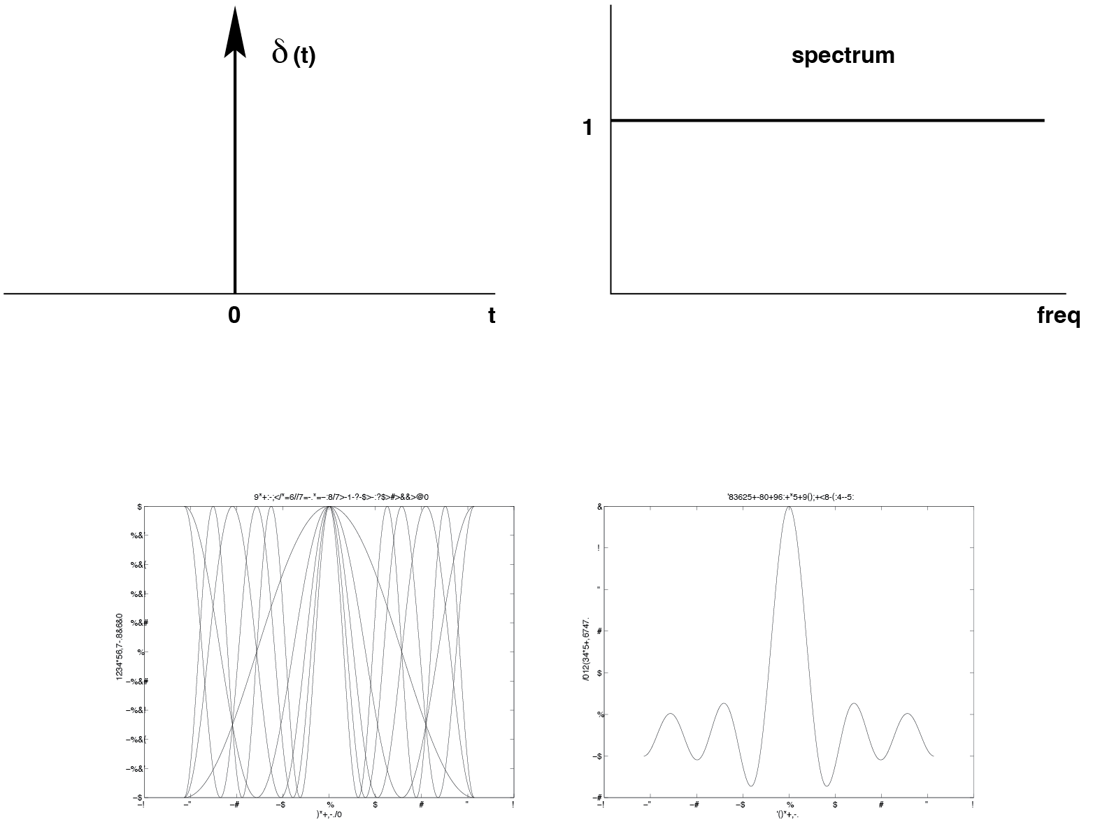
Fig. 5 A. The impulse in the time domain and the associated spectrum. B: One can clearly see how summation of five cosines (which are in phase), already gives rise to a sharp peak (height 5) around t = 0.

A very important example within this category of signals is the Dirac impulse function (called after the mathematician Paul Dirac, Fig. 5). This is one of the most commonly used signals in systems theory, especially because of the convenient mathematical properties of such a signal. The how and why of this comes next and will be extensively discussed. The impulse function, \(\delta (t)\), is defined by:

(8)\[\begin{split}\begin{split} \delta(t) & = \infty \text{ for } t = 0 \\ & = 0\text{ for } t \neq 0 \\ \text{ with } \int_{-\infty}^{+\infty} \delta t dt & = 1 \text{ (surface area = 1)} \\ \text{ such that } \int_{-\infty}^{+\infty} f(t) \cdot \delta (t-t_0) & = f(t_0) \end{split}\end{split}\]

The impulse function, often denoted as (\delta(t)), is a mathematical function that is zero everywhere except at (t = 0), where it is infinitely high and has an integral of one. Especially the last property (superposition) will prove to be of great importance for the description of linear systems. Check for yourself that the last property follows from the third.

Impulse Decomposition

Impulse decomposition refers to the process of breaking down a signal into a series of impulses (or delta functions) and their associated coefficients. This concept is rooted in the idea that many signals can be represented as a sum of scaled and shifted impulses (superposition).

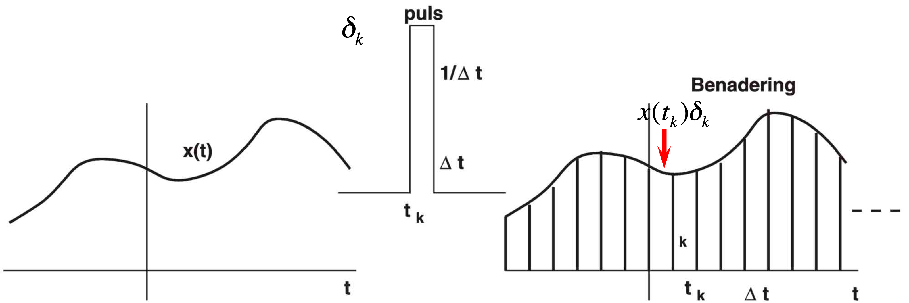
Fig. 6 Any signal \(x(t)\) can be described as a sequence of pulses with variable height.

How Impulse Decomposition Works

• Representation: A signal (x(t)) is represented as a sum of impulses: (x(t) = \sum a_n \delta(t - t_n)), where (a_n) are coefficients, and (t_n) are the time-shifts of the impulses (Fig. 6).

• Decomposing Complex signals: This approach decomposes a complex signal into simpler elements (impulses), making analysis easier. It’s particularly useful in systems where the response to an impulse input can be used to characterize the entire system.

• Neural Spike Analysis: In neuroscience, impulse decomposition can be applied to represent neural spike trains, where each spike is modeled as an impulse.

Key Insight: Any signal can always be approximated by a sum of pulses with variable height.

Exercises

In this module, we were introduced to the concept of signals, and to the idea of time domain and frequency domain representations of signals. In particular, we learned about the Fourier theorem for periodic functions. We are now first trying to familiarize ourselves (a little bit) with an example of Fourier analysis, by applying it to a couple of very simple functions.

exercise - factorial

Recall that \(n!\) is read as “\(n\) factorial” and defined as \(n! = n \times (n - 1) \times \cdots \times 2 \times 1\).

There are functions to compute this in various modules, but let’s write our own version as an exercise.

In particular, write a function factorial such that factorial(n) returns \(n!\) for any positive integer \(n\).

exercise - periodic function 1

Compute the Fourier coefficients for the following periodic function:

\[\begin{split}x(t)=\begin{cases} +1, & \text{if $0\leq t < 1$}.\\ -1, & \text{if $-1\leq t < 0$}. \end{cases}\end{split}\]

and \(x(t)\) is periodic.

• What is its period?

• Is it even/odd?

• Determine \(a_n\) and \(b_n\), and \(c_n\) and \(\phi_n\)

• Plot the spectrum of \(x(t)\).

exercise - periodic function 2

Compute the Fourier coefficients for the following periodic function:

\[\begin{split}x(t)=\begin{cases} +1, & \text{if $0\leq t < 2$}.\\ 0, & \text{if $-2\leq t < 0$}. \end{cases}\end{split}\]

and \(x(t)\) is periodic.

• What is its period?

• Use a clever trick to make it an even function

• Determine \(a_n\) and \(b_n\), and \(c_n\) and \(\phi_n\)

• Plot the spectrum of \(x(t)\).

exercise - Dirac

We discussed the Dirac delta function. This (idealized) function turns out to be a crucial input signal to study linear systems in the time domain (next lectures). It is also called the ‘impulse function’. In this exercise we practice the idea that this function is zero everywhere, except when it’s argument is zero:

\[\begin{split}\delta(x)=\begin{cases} \infty, & \text{if $x=0$}.\\ 0, & \text{otherwise}. \end{cases}\end{split}\]

Draw the following functions.

• \(\delta(2x)\)

• \(\delta(x^2)\)

• \(\delta(a \cdot x^n)\) with \(a>0\)

• \(\delta(e^x)\)

• \(\delta(x+a)\)

• \(\delta(x-a)\)

• \(\delta(t^2-5t+6)\)

• \(\delta(\sin{(10t)} \cdot \cos{(10t)})\)

exercise - synthesis

Given eqns. eqn_synthesiseqn and eqn_afourierserieseqn, show that it is possible to rewrite to eqn. eqn_trigeqn:

\[a_n \cdot \cos{(n \omega_0 t)} + b_n \cdot \sin{(n \omega_0 t)} = c_n \cdot \cos{(n \omega_0 t+\phi_n)}.\]

• To show this you have to show for which values of \( a_n \) and \( b_n \) this relationship holds. What are those values in terms of \(c_n \) and \(\phi_n \)?

• What are \( c_n \) and \( \phi_n \) in terms of \(a_n \) and \(b_n \)?

Hint: use \(\cos{(x+y) = \cos{(x)}\cos{(y)}-\sin{(x)}\sin{(y)}}\) (e.g. see the list on trigonometric identities on Wikipedia).

exercise - frequency resolution

We have also seen (Powerpoint file) that according to Fourier analysis there exists a fundamental inverse relationship between the resolutions (i.e., precision) of a signal’s representation in the time domain and the frequency domain. This relationship was expressed by:

\[\Delta T \cdot \Delta f \approx 1\]

In words: Events that are defined very precisely in the time domain (e.g. a sharp onset and short duration, a brief pulse, etc.) have a very broad representation in the frequency domain (i.e. they are broadband). On the other hand, signals that are defined very precisely in the frequency domain (e.g. a pure tone) have a very broad representation (i.e. a very long duration) in the time domain (i.e., their on- and offsets are poorly defined). We now derive this very important relation (fundamental to signal analysis) for the following periodic function:

\[\begin{split}x(t)=\begin{cases} +1, & \text{if $0\leq t < \Delta T$}.\\ 0, & \text{if $\Delta T \leq t < T$}. \end{cases}\end{split}\]

where \(\Delta T \ll T\) and \(x(t)\) is periodic.

• What is its period?

• What clever trick can you do to make it an even function?

• Determine \(a_n\) and \(b_n\), and \(c_n\) and \(\phi_n\)

• Plot the spectrum of this function as a function of n for different relative pulse duration, \(\frac{\Delta T}{T} = 0.05, 0.1, 0.2,\) and \(0.5\).

exercise - time-frequency

We next apply the time-frequency duality concept to an exponentially decaying pulse (i.e., a continuous function), which is defined by:

\[x(t) = A \cdot \exp{(\frac{-t}{T})}\]

• Draw a graphical representation of this function for \(T=0.2, 0.5\) and \(1.0\) s. \(T\) is the so-called time constant of this function.

• Give the mathematical description of the tangent to this function in \(t=0\).

• Sketch the function and the tangent.

• Determine at which moment in time the tangent crosses the \(x=0\) axis

• Sketch in a different graph (no need to compute) the spectra for the three functions in a.

Learning goals

Learning Outcomes

To understand why the sensorimotor systems process signals in the way they do, we need to cover some elementary background of signal analysis (Signals, Assignment: Fourier decomposition, and Application: Analyzing Voices). This module presents the foundation of signals analysis. We will cover various types of signals (Dirac impulses and harmonics) and various ways for breaking signals into simpler components (impulse responses in the time domain, representation in the frequency domain). At the end of this modules, you will be able to:

• Provide definitions of signals, Dirac pulse, impulse, Fourier, harmonic,

• Explain impulse and Fourier decomposition

Key Concepts

• signals are a description of how one parameter varies with another (e.g. pressure as a function of time).

• signals can be viewed as a superposition (sum) of simpler signals.

• We can decompose an input signal into a group of simpler components (Dirac impulses or sines and cosines).

Key Terms

signal

a description of how one parameter varies with another (e.g. pressure as a function of time)

continuous

a continuous signal is defined for every value of time and can take on any value.

discrete

a discrete signal is defined only at specific time intervals and takes on discrete values. It’s often a result of sampling a continuous signal.

periodic

a periodic signal repeats its pattern over a fixed, regular interval, known as the period.

aperiodic

an aperiodic signal does not repeat its pattern over regular intervals. Its pattern may or may not be predictable but does not exhibit periodicity.

impulse

a signal composed of all zeros except a single nonzero point

Delta function

a normalized impulse – a signal with an amplitude at t=0 and is 0 otherwise, with an area of 1

decomposition

the process of breaking a signal down into simpler or more fundamental parts

Fourier analysis

mathematical techniques based on decomposing signals into sinusoids

Fourier series

Fourier analysis for periodic, continuous signals (cf discrete Fourier transform, Fast Fourier Transform)