Assignment: The Nonlinear Burst Generator

Assignment: The Nonlinear Burst Generator#

Learning Goals#

Learning Goals — Assignment: Nonlinear Burst Generator

After completing this assignment, you should be able to:

Explain the functional roles of the Burst Generator, Neural Integrator, Direct Path, Feedback Loop, OPNs, and Oculomotor Plant, and describe their interactions in producing a saccade.
Describe the nonlinear properties of the burst generator (saturation, angular constant) and how these shape saccade kinematics.
Explain inverse reconstruction, including the role of high-gain feedback in recovering the motoneuron command from eye-movement data.
Interpret main-sequence relationships and how model parameters determine peak velocity and duration as a function of amplitude.
Explain how OPN timing and feedback gain influence saccade onset, peak velocity, overshoot, and accuracy.
Understand the functional interpretation of SC bursts, distinguishing effects of burst height, duration, and spike count.
Relate CNS parameter manipulations to pharmacological effects, such as slowed, more variable saccades under Valium while plant mechanics remain unchanged.
Identify which components control amplitude, which shape kinematics, and which maintain accuracy.
Explain why accuracy may be preserved even when kinematics slow significantly.
Relate the model outputs to empirical human saccade data, including increased variability or pharmacological perturbations.
Evaluate whether a set of CNS changes can explain observed behavioral outcomes, using control-theoretic reasoning.

Data#

Downloads#

Download the Matlab files:

Matlab Code for Saccade Model.

This contains the saccade model, which contains the burst generator of the saccadic system as discussed in The Saccadic System - The Burst Generator.

Research Data Management#

To keep your work organised and reproducible, set up a simple folder structure before you begin:

Create a main folder named NBP_burst.
Inside this folder, create three subfolders:
- data – for storing exported simulation data files
- analysis – for your MATLAB scripts and the Simulink model
- figures – for saving plots and exported images

Place the Simulink model and all MATLAB code in the analysis folder. Then create a new MATLAB script named data_analysis.m in this folder. You will use this script to run your simulations, analyse the output, and generate figures. Whenever your script produces data files or images, save them into the corresponding data or figures folder. This structure helps ensure your work is easy to navigate, reproducible, and ready for future assignments. For additional guidance, see Research Data Management.

Working With Simulink#

This practical uses Simulink. Simulink is MATLAB’s graphical environment for building and simulating dynamic systems. Instead of writing equations in code, you create models by connecting functional blocks that represent mathematical operations, neural circuits, or physical systems. Many biological systems—including the saccadic pulse–step generator—can be described as continuous-time, dynamic systems with:

inputs (e.g., neural pulse signals)
internal computations (e.g., integration, time constants)
outputs (e.g., eye position and velocity)

Simulink lets you:

visualize the components (neurons, integrators, plant dynamics)
modify parameters interactively
see the consequences immediately in scopes
simulate continuous time without manually coding differential equations

This makes it ideal for understanding how the brain generates precise movements.

Opening the Model#

Start MATLAB.
In the Command Window, type (or put this in a script and run that script):

   open_system("saccade.slx")

Note: the first exercise will make use of the pulsestep.slx model.

The top-level Simulink diagram will open.

Running Simulations#

Click Run ( ▶ ) in the Simulink toolbar.
The default simulation time is 0.5 s, which is appropriate for saccades.

Viewing Signals#

After clicking Run, Scopes will appear that contain the signals generated by the simulation.

Editing Parameters#

Double-click any subsystem block:

Burst Generator
LLBN
Feedback
Synaptic gain
OPNs
SC burst

Then edit the parameters (e.g., Bmax, A0 of the Burst Generator block, FR, D of the SC block).
Use correct units: seconds, milliseconds, spikes/s, dimensionless gains.

Creating a Figure#

To create a figure of a Scope in a Word-document, you can right-click on the scope and choose “Print Display to Figure”, which creates a Matlab Figure. You can copy that figure (click on Figure>Copy Figure) and paste this into the Word-document.

MATLAB#

In this tutorial, you will receive MATLAB code that automates the simulations required for each assignment. However, make sure to actively explore the Simulink model yourself:

double-click blocks to inspect and change parameters,
view and measure the signals in the Scopes or Data Inspector,
and reason about how each subsystem affects the final eye-movement output.

The goal is not only to run the scripts, but to understand how this model represents the final stages of the saccadic system, and how changes in pulse, step, and plant dynamics shape the behavior of real saccades.

Computer exercises with the nonlinear Burst generator model#

These exercises introduce you to the behaviour of the burst generator, including feedback and nonlinearity. We will inspect a simple model of the so-called ‘Final Common Pathway’ of the oculomotor system including the burst generator (Fig. 74) is also available under Simulink as file saccade.slx (Fig. 51 and Fig. 52). This simulation model, allows you to interactively set parameters of:

The saccadic burst from the EBNs/IBNs (this is simply modeled as a pulse, having a height, \(P\), and duration \(D\).)
The neural integrator: setting its gain to zero mimics total loss of the integrator, whereas a gain of one means normal operation.
The direct path: feeds the pulse directly to the oculomotor neurons. When its gain is set to zero, you actually simulate the effect of a Step input to the OMNs.
The Plant, with its two time constants, \(T_1\) and \(T_2\)

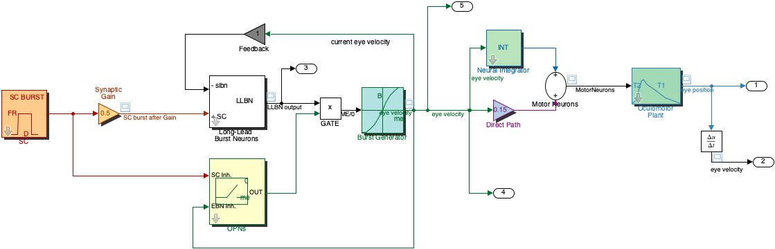
../_images/saccademodel.png — Fig. 74 | Saccadic System Model including the Burst Generator#

This model includes the nonlinear burst generator (EBNs/IBNs).

Exercise 8 — Pulse–Step Reconstruction#

In this exercise we investigate how the inverse plant reconstructs the motoneuron pulse–step command from the eye-position signal.

Task#

Run the default Pulse–Step model pulsestep.slx.

%% Pulse–Step Generator – MATLAB/Simulink Helper Script
% This script loads the Simulink model 'pulsestep.slx', sets parameters,
% runs simulations, and extracts the logged signals EyePos, EyeVel, Command.

clear; close all; clc;

modelName = "pulsestep";

%% 1. Load and open the model
load_system(modelName);
open_system(modelName);


%% 2. Set default parameter values
psg_set_default_params(modelName);

%% PRESS RUN

Plot both:
- the original pulse–step command (the signal driving the plant),
- the reconstructed pulse–step command (output of the Inverse Plant Model).
Answer the following:
- How similar are they?
- Where do small differences appear?
- Explain why reconstruction works (e.g. Fig. 75). To answer this open the Inverse Plant Model block by right-clicking on it → Mask → Look Under Mask. Inside, you will find two key components: a. A copy of the oculomotor plant, with the same time constants \(T_1\) and \(T_2\). b. A high-gain negative-feedback loop (with gain \(K = 2000\)).
- i.e. why does feedback enable reconstruction?
- Does this require full knowledge of plant parameters?
- Why are the reconstructed and original commands not identical?

Note - Transfer Characteristic block

Note: Why is there a small filter after the inverse model?

If you look inside the Inverse Plant Model (right-click → Look Under Mask), you will see a final Transfer Fcn block with:

Numerator: [1]
Denominator: [0.008 1]

This block is a first-order low-pass filter with a time constant of:

\(\tau = 0.008 \text{ s (8 ms)}\).

Its role is to smooth the reconstructed pulse–step command. The inverse model (which uses a high-gain feedback loop and a copy of the plant dynamics) effectively computes something close to the mathematical inverse of the oculomotor plant. Inverting a low-pass system behaves a bit like differentiation, which can amplify very high-frequency noise.

The small 8-ms low-pass filter therefore:

suppresses numerical noise from the inverse operation,
prevents extremely sharp, unrealistic spikes in the reconstructed signal,
keeps the reconstructed pulse–step biologically plausible.

In summary:

The filter stabilizes and smooths the reconstructed command by removing the high-frequency noise that naturally appears when inverting a low-pass plant.

Explain why small differences exist.

MATLAB Code

%% Exercise 8 — Pulse–Step Reconstruction
% Goal:
%   - Run the model with default parameters
%   - Plot the ORIGINAL pulse–step command
%   - Plot the RECONSTRUCTED pulse–step from the inverse plant
%   - Visually compare them
%
% NOTE:
%   You may need to adapt the column indices for y(:,k) depending on
%   how your model outputs are ordered (see comments below).

disp('Exercise 8 — Pulse–Step Reconstruction');

% --- 1. Set model to default parameters (adapt if you have a helper) ---
% If you created a set_default_params(modelName) function, you can just call:
psg_set_default_params(modelName);
% Otherwise, set key defaults here explicitly:


% --- 2. Run the simulation with default settings ---
simOut = sim(modelName);

t = simOut.tout;
y = simOut.yout;   % numeric matrix with model outputs (columns)

% --- 3. Extract original and reconstructed pulse–step signals ---
% IMPORTANT:
%   Adjust these indices to match your model:
%   - originalIdx: column containing the ORIGINAL pulse–step command
%   - reconIdx:    column containing the RECONSTRUCTED pulse–step
%
% Look at your model's Outport blocks (or To Workspace blocks) to see
% which output corresponds to which signal.
%
% Example (you can start with this guess and adjust if needed):
originalIdx = 7;   %
reconIdx    = 3;   %

origPulse = y(:, originalIdx);
recPulse  = y(:, reconIdx);

% --- 4. Plot original vs reconstructed pulse–step ---
figure(13);
clf
plot(t, origPulse, 'LineWidth', 1.5);
hold on;
plot(t, recPulse, '--', 'LineWidth', 1.5);
xlabel('Time (s)');
ylabel('Command (a.u.)');
title('Original vs reconstructed pulse–step command');
legend({'Original pulse–step', 'Reconstructed pulse–step'}, 'Location', 'Best');
grid on;

% --- 5. Simple quantitative comparison (optional) ---
% Correlation and mean absolute difference
valid = ~isnan(origPulse) & ~isnan(recPulse);
corrCoeff = corr(origPulse(valid), recPulse(valid));
madDiff   = mean(abs(origPulse(valid) - recPulse(valid)));

fprintf('Correlation between original and reconstructed command: %.3f\n', corrCoeff);
fprintf('Mean absolute difference: %.3g (arbitrary units)\n', madDiff);

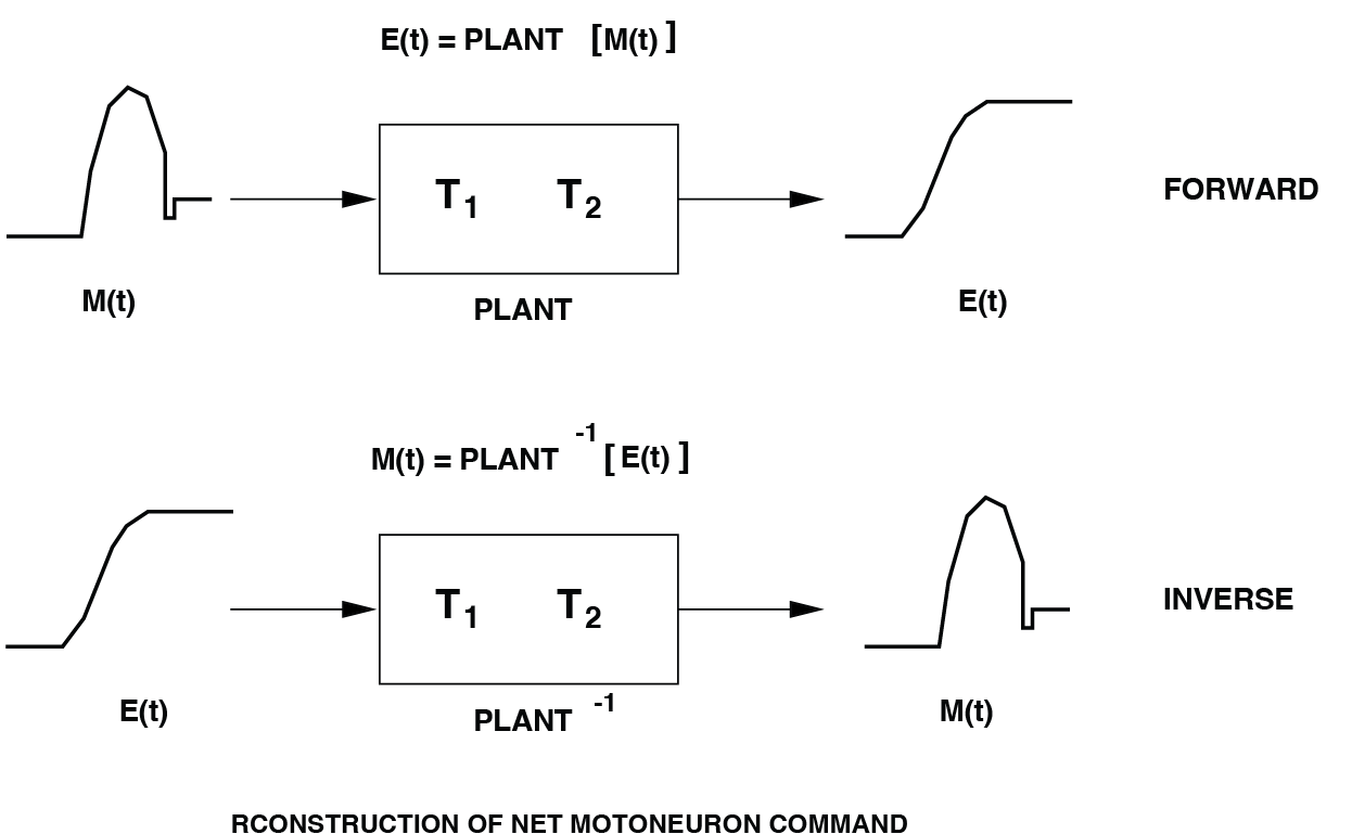
../_images/omnreconstruction.png — Fig. 75 By virtue of the plant’s linearity, it is possible to reconstruct an estimate of its net neural pulse-step control signal from the measured eye movement, \(E(t)\).#

Exercise 9 - amplitude#

Now we continue with the Saccade model saccade.slx with its default parameter set (these are already set, see Table 1).

clear; close all; clc;

modelName = "saccade";

%% 1. Load and open the model
load_system(modelName);
open_system(modelName);


%% 2. Set default parameter values
saccade_set_default_params(modelName);

%% PRESS RUN

Then change the saccade amplitude by changing the value of the Synaptic Gain block to 1.0 (the Synaptic Gain the connection strength of a particular SC site to the saccade generator).

How is saccade amplitude related to the Synaptic Gain?
How would you obtain saccade amplitudes of 1, 5, 10, 20, and 30 deg?

Hint

Because the Synaptic Gain block represents a linear mapping from SC activity to burst-generator input, saccade amplitude scales linearly with Synaptic Gain. Therefore, measuring amplitude at one known gain allows you to analytically compute the required gain for any desired amplitude.

You can and should verify this!

Table 1 Parameters of the Simulink saccade model#
Stage	Symbol	Meaning	Range	Default	Unit
SC	FR	firing rate, burst height	[0 – 1000]	800	Hz
	D	burst duration	[0 – 0.20]	50	ms
Synaptic Gain	R	SC–BS connection strength	[0.1 – 1.5]	0.5	–
Burst Generator	Bmax	pulse height max	[0 – 1000]	700	deg/s
	A0	angular constant	[1 – 100]	7	deg/s
OPNs	Bias	fixation OPN firing rate	[50 – 500]	80	Hz
	Delay	trigger moment from SC	[0 – 50]	15	ms
	SC Gain	attenuates SC burst	[0 – 1]	0.2	–
Feedback Path	Gain (K)	feedback gain	[0 – 5]	1.0	–
Neural Integrator	G	integrator gain	[0 – 1.0]	1.0	–
Direct Path	Gain (K)	forward gain	[0 – 0.5]	0.15	–
Oculomotor Plant	T1	long time constant	[0.05 – 0.30]	0.15	s
	T2	short time constant	[0 – 0.03]	0.020	s

MATLAB Code

%% Exercise 9 — Amplitude control by Synaptic Gain
% Goal:
%   - Demonstrate that Synaptic Gain scales the saccade amplitude linearly.
%   - Use one calibration measurement to compute gain values for any amplitude.

disp('Exercise 9 — Amplitude and Synaptic Gain');

%% ------------------------------------------------------------------------
% 1. Load default model parameters
% -------------------------------------------------------------------------
saccade_set_default_params(modelName);

% Choose a calibration Synaptic Gain (e.g., 0.5)
SG_calib = 0.5;
% set_param(modelName + "/Synaptic Gain", "Gain", num2str(SG_calib));  % adjust mask name if needed

% Run model once at calibration gain
simOut = sim(modelName);
t = simOut.tout;
y = simOut.yout;

% Extract eye position (adjust index if needed)
EyePos = y(:,1);

% Measured calibration amplitude
Amp_calib = EyePos(end) - EyePos(1);

fprintf('Calibration amplitude = %.3f deg at Synaptic Gain = %.3f\n', ...
        Amp_calib, SG_calib);

% Linear scaling slope:
%     amplitude = slope * SynapticGain
slope = Amp_calib / SG_calib;
fprintf('Slope = %.3f deg/unit gain\n', slope);

%% ------------------------------------------------------------------------
% 2. Compute Synaptic Gain required for specific target amplitudes
% -------------------------------------------------------------------------
desiredAmp = [1 2 5 10 20 30];   % desired saccade amplitudes
nA = numel(desiredAmp);

SG_required = desiredAmp / slope;    % since amplitude ≈ slope * Gain

Amp_actual  = zeros(1, nA);

% Validate these gains by running the model
for i = 1:nA
    SG = SG_required(i);
    set_param(modelName + "/Synaptic Gain", "Gain", num2str(SG));

    simOut = sim(modelName);
    y = simOut.yout;
    EyePos = y(:,1);

    Amp_actual(i) = EyePos(end) - EyePos(1);
end

%% -------------------------------------------------------------------------
% 3. Plot desired vs measured amplitudes (should lie on unity line)
% -------------------------------------------------------------------------
figure;
plot(desiredAmp, Amp_actual, 'ko-', ...
     'LineWidth', 1.5, 'MarkerSize', 21, 'MarkerFaceColor', 'w');
hold on;
refline(1,0);   % unity line
xlabel('Desired amplitude (deg)');
ylabel('Measured amplitude (deg)');
title('Amplitude control via Synaptic Gain (linear relationship)');
xlim([-2 32]); ylim([-2 32]);
grid on;

if exist('nicegraph')
nicegraph;  % optional formatting function
end

Exercise 10 — Main Sequence#

In this exercise, you will examine how the main sequence (the relationship between saccade amplitude, peak velocity, and duration) is affected by the Burst Generator. First, ensure that the parameters of the Pulse–Step part of the model (Neural Integrator, Direct Path, Oculomotor Plant), the Burst Generator, and the Superior Colliculus (SC) are all set to their default values (see Table Table 1 for saccade.slx).

You will generate saccades of different amplitudes (1, 5, 10, 20, and 30 deg), and for each saccade you will measure:

Amplitude (final eye position minus initial position)
Peak velocity (maximum of the eye-velocity trace)
Duration (time interval during which eye velocity exceeds ~10% of its peak)

You can obtain these measures either:

manually from the Scope using cursors/rulers (do this at least once), or
automatically in MATLAB (see example code).

Then:

Normal main sequence
Obtain the main sequence for normal saccades (default Burst Generator: Bmax = 700 deg/s, A0 = 7 deg).
Generate saccades with amplitudes of approximately 1, 5, 10, 20, and 30 deg.
Effect of Burst saturation (Bmax)
Change the Burst Generator saturation level Bmax to 1400 deg/s and then to 1350 deg/s, and determine the main sequence again.
Effect of angular constant (A0)
Change the Burst Generator angular constant A0 to 2 deg and then to 28 deg, and determine the main sequence again.
Question
How do changes in Burst Generator parameters (Bmax and A0) affect:
- the shape and slope of the main sequence,
- the relationship between amplitude and duration,
- and the saturation behaviour at large amplitudes?

Make plots of:

peak velocity vs. amplitude, and
duration vs. amplitude

for all parameter settings in a single figure (use different colours/markers and a clear legend).

MATLAB Code

%% Exercise 10 — Main Sequence (Burst Generator effects)
% We will:
%   - compute the main sequence (peak velocity and duration vs amplitude)
%     for different Burst Generator parameters (Bmax, A0)
%   - generate saccades of approximately [1 5 10 20 30] deg
%     by adjusting the Synaptic Gain.

disp('Exercise 10 — Main Sequence and Burst Generator parameters');

modelName = "saccade";

% Desired saccade amplitudes (deg)
targetAmps = [1:3:30];
nA         = numel(targetAmps);

% Define conditions for the Burst Generator
% Default: Bmax = 700, A0 = 7
conditions = struct( ...
    "name",   { "Default",      "Bmax = 1400",    "Bmax=350",    "A0=2",        "A0=28" }, ...
    "Bmax",   {     700,    350,	1400,   700,  700 }, ...
    "A0",     {		7,		7,      7,		2,    28 } ...
    );

nCond = numel(conditions);

% Storage for main sequence data
Amp_all   = nan(nCond, nA);
Vpeak_all = nan(nCond, nA);
Dur_all   = nan(nCond, nA);

for c = 1:nCond
    cond = conditions(c);
    fprintf('\nCondition: %s (Bmax=%.0f, A0=%.1f)\n', cond.name, cond.Bmax, cond.A0);

    % -------------------------------------------------------------
    % 1. Reset model to defaults and apply Burst Generator settings
    % -------------------------------------------------------------
    saccade_set_default_params(modelName);

    % Set Burst Generator parameters for this condition
    set_param(modelName + "/Burst Generator", ...
        "Bmax", num2str(cond.Bmax), ...
        "Ao",   num2str(cond.A0));

    % -------------------------------------------------------------
    % 2. Calibrate Synaptic Gain for this condition
    % -------------------------------------------------------------
    % Choose a calibration gain (e.g., 0.5) and see what amplitude we get.
    SG_calib = 0.5;
    set_param(modelName + "/Synaptic Gain", "Gain", num2str(SG_calib));

    simOut = sim(modelName);
    t = simOut.tout;
    y = simOut.yout;

    EyePos = y(:,1);
    EyeVel = y(:,2);

    [Amp_calib, Vpeak_calib, Dur_calib] = saccade_measure(t, EyePos, EyeVel);

    fprintf('  Calibration amplitude: %.2f deg at Synaptic Gain R=%.2f\n', ...
        Amp_calib, SG_calib);

    % Assume amplitude scales approximately linearly with R for this condition:
    %     Amp ≈ slope * R    =>    slope ≈ Amp_calib / SG_calib
    slope = Amp_calib / SG_calib;

    % -------------------------------------------------------------
    % 3. Generate saccades at target amplitudes
    % -------------------------------------------------------------
    for i = 1:nA
        A_target = targetAmps(i);

        % Approximate Required R (may not be exact at large amplitudes)
        R_needed = A_target / slope;
        set_param(modelName + "/Synaptic Gain", "Gain", num2str(R_needed));

        simOut = sim(modelName);
        t = simOut.tout;
        y = simOut.yout;

        EyePos = y(:,1);
        EyeVel = y(:,2);

        [Amp, Vpeak, Dur] = saccade_measure(t, EyePos, EyeVel);

        Amp_all(c,i)   = Amp;
        Vpeak_all(c,i) = Vpeak;
        Dur_all(c,i)   = Dur;

        fprintf('    Target %.1f deg -> R≈%.3f, Amp=%.2f deg, Vpeak=%.1f deg/s, Dur=%.1f ms\n', ...
            A_target, R_needed, Amp, Vpeak, Dur*1000);
    end
end

pause(1);

%% -------------------------------------------------------------
% 4. Plot main sequences for all conditions
% --------------------------------------------------------------
cols = lines(nCond);   % colour map

% Peak velocity vs amplitude
figure;
subplot(1,2,1);
hold on;
for c = 1:nCond
    plot(Amp_all(c,:), Vpeak_all(c,:), 'o-', ...
        'Color', cols(c,:), 'LineWidth', 1.5, 'DisplayName', conditions(c).name);
end
xlabel('Saccade amplitude (deg)');
ylabel('Peak velocity (deg/s)');
title('Main sequence: peak velocity vs amplitude');
grid on;
legend('Location','best');
axis square

% Duration vs amplitude
subplot(1,2,2);
hold on;
for c = 1:nCond
    plot(Amp_all(c,:), Dur_all(c,:)*1000, 'o-', ...
        'Color', cols(c,:), 'LineWidth', 1.5, 'DisplayName', conditions(c).name);
end
xlabel('Saccade amplitude (deg)');
ylabel('Duration (ms)');
title('Main sequence: duration vs amplitude');
grid on;
legend('Location','best');

axis square;

Exercise 11 — Influence of the Feedback Gain#

In this exercise you will investigate how the feedback gain in the brainstem loop affects the dynamics of a saccade.

Start from the default parameter set of the saccade.slx model
(see Table Table 1 and use saccade_set_default_params).
First generate a reference saccade of ~20° amplitude using the default settings
(including the default Feedback Path gain K = 1.0).
Note the eye-position and eye-velocity traces.
Next, vary the Feedback Path gain to:
- K = 0.5
- K = 1.0 (default)
- K = 2.0
For each value of K, simulate the model with the same Synaptic Gain as in the reference condition and plot:
- eye position as a function of time
- eye velocity as a function of time
Compare the traces across feedback gains:
- How do rise time, peak velocity, and overshoot change?
- Does the eye reach the same final position?
- Does a higher feedback gain make the system faster, more accurate, or less stable?

Explain the resulting effects in terms of feedback control:
how increasing or decreasing the loop gain changes the correction of motor error and the stability of the eye-movement system.

MATLAB Code

%% Exercise 11 — Influence of the Feedback Gain
% We:
%   - Start from default parameters
%   - Calibrate a ~20 deg saccade with default feedback gain K = 1.0
%   - Then vary Feedback Path gain K = [0.5, 1.0, 2.0] using the same
%     Synaptic Gain and compare eye position and velocity traces.

disp('Exercise 11 — Influence of the Feedback Gain');

modelName = "saccade";

% -------------------------------------------------------------
% 1. Set defaults and calibrate a ~20 deg saccade for K = 1.0
% -------------------------------------------------------------
saccade_set_default_params(modelName);

% Ensure Feedback Path gain is at default
K_default = 1.0;
set_param(modelName + "/Feedback", "Gain", num2str(K_default));

% Choose a starting Synaptic Gain and calibrate to ~20 deg
SG0 = 0.5;   % initial guess
set_param(modelName + "/Synaptic Gain", "Gain", num2str(SG0));

simOut = sim(modelName);
t = simOut.tout;
y = simOut.yout;

EyePos = y(:,1);
EyeVel = y(:,2);

Amp0 = EyePos(end) - EyePos(1);
Vpeak0 = max(EyeVel);

targetAmp = 20;  % desired reference amplitude (deg)

% Approximate linear scaling of Synaptic Gain to reach targetAmp
scaleSG = targetAmp / Amp0;
SG_ref  = SG0 * scaleSG;

set_param(modelName + "/Synaptic Gain", "Gain", num2str(SG_ref));

% Run once more with calibrated Synaptic Gain at K = 1.0
simOut = sim(modelName);
t = simOut.tout;
y = simOut.yout;

EyePos = y(:,1);
EyeVel = y(:,2);

Amp_ref   = EyePos(end) - EyePos(1);
Vpeak_ref = max(EyeVel);

fprintf('Reference condition (K=%.1f): SG=%.3f -> Amp ≈ %.2f deg, Vpeak ≈ %.1f deg/s\n', ...
    K_default, SG_ref, Amp_ref, Vpeak_ref);

% -------------------------------------------------------------
% 2. Vary Feedback Path gain: K = 0.5, 1.0, 2.0
% -------------------------------------------------------------
K_values = [0.5 1.0 2.0];
nK       = numel(K_values);

% Store trajectories for plotting
EyePos_all = cell(1, nK);
EyeVel_all = cell(1, nK);
t_all      = cell(1, nK);
Amp_all    = zeros(1, nK);
Vpeak_all  = zeros(1, nK);

for i = 1:nK
    K = K_values(i);
    set_param(modelName + "/Feedback", "Gain", num2str(K));

    % Use the same Synaptic Gain as reference (SG_ref)
    set_param(modelName + "/Synaptic Gain", "Gain", num2str(SG_ref));

    simOut = sim(modelName);
    t = simOut.tout;
    y = simOut.yout;

    EyePos = y(:,1);
    EyeVel = y(:,2);

    t_all{i}      = t;
    EyePos_all{i} = EyePos;
    EyeVel_all{i} = EyeVel;

    Amp_all(i)   = EyePos(end) - EyePos(1);
    Vpeak_all(i) = max(EyeVel);

    fprintf('K=%.1f -> Amp=%.2f deg, Vpeak=%.1f deg/s\n', ...
        K, Amp_all(i), Vpeak_all(i));
end

% -------------------------------------------------------------
% 3. Plot eye position and velocity traces for all K
% -------------------------------------------------------------
cols = lines(nK);

figure;
subplot(2,1,1);  % Eye position
hold on;
for i = 1:nK
    plot(t_all{i}, EyePos_all{i}, 'LineWidth', 1.5, ...
        'Color', cols(i,:), 'DisplayName', sprintf('K=%.1f', K_values(i)));
end
xlabel('Time (s)');
ylabel('Eye position (deg)');
title('Effect of Feedback Gain on Eye Position (reference ~20° saccade)');
grid on;
legend('Location','best');

subplot(2,1,2);  % Eye velocity
hold on;
for i = 1:nK
    plot(t_all{i}, EyeVel_all{i}, 'LineWidth', 1.5, ...
        'Color', cols(i,:), 'DisplayName', sprintf('K=%.1f', K_values(i)));
end
xlabel('Time (s)');
ylabel('Eye velocity (deg/s)');
title('Effect of Feedback Gain on Eye Velocity');
grid on;
legend('Location','best');

Exercise 12 — Influence of OPN Timing#

In this exercise you will investigate how the timing of the OmniPause Neurons (OPNs) affects:

the LLBN burst (shape, onset, and duration), and
the kinematics of the resulting 20° saccades.

Start from the default parameter set of saccade.slx
(use saccade_set_default_params, see Table Table 1).
First, with the default OPN delay (e.g. Delay = 15 ms), adjust the Synaptic Gain so that the model generates a saccade of about 20°.
Now keep this Synaptic Gain fixed, and only change the OPN delay (the SC-trigger delay in the OPN block) to:
- 10 ms
- 15 ms (default)
- 25 ms
For each delay:
- simulate the model,
- plot eye position and eye velocity as a function of time,
- plot the LLBN burst as a function of time.
Describe how changing the OPN delay affects:
- the onset time, peak, and duration of the LLBN burst,
- the peak velocity, duration, and accuracy (final position) of the saccades.
Explain your observations.
(Hint: look under the LLBN mask and identify how and when the feedback term is added. How does the OPN timing change the moment at which feedback “kicks in” and starts shaping the burst?)

MATLAB Code

%% Exercise 12 — Influence of OPN timing
% Goal:
%   - Study how OPN delay (SC-trigger timing) changes the LLBN burst
%     and saccade kinematics for ~20 deg saccades.

disp('Exercise 12 — OPN timing and LLBN burst');

modelName = "saccade";

% -------------------------------------------------------------
% 1. Set defaults and calibrate a ~20 deg saccade at default OPN delay
% -------------------------------------------------------------
saccade_set_default_params(modelName);

% Default OPN delay (ms) — check table / mask:
Delay_default_ms = 15;       % as in your assignment
set_param(modelName + "/OPNs", "DEL", num2str(Delay_default_ms));

% Initial guess for Synaptic Gain
SG0 = 0.5;
set_param(modelName + "/Synaptic Gain", "Gain", num2str(SG0));

% Run once
simOut = sim(modelName);
t = simOut.tout;
y = simOut.yout;

% Extract eye position and velocity [adjust indices if needed]
EyePos = y(:,1);
EyeVel = y(:,2);

Amp0   = EyePos(end) - EyePos(1);
Vpeak0 = max(EyeVel);

targetAmp = 20;  % desired amplitude in degrees

% Simple linear calibration of Synaptic Gain
scaleSG = targetAmp / Amp0;
SG_ref  = SG0 * scaleSG;

set_param(modelName + "/Synaptic Gain", "Gain", num2str(SG_ref));

% Re-run with calibrated Synaptic Gain at default OPN delay
simOut = sim(modelName);
t = simOut.tout;
y = simOut.yout;

EyePos = y(:,1);
EyeVel = y(:,2);

Amp_ref   = EyePos(end) - EyePos(1);
Vpeak_ref = max(EyeVel);

fprintf('Reference (Delay=%d ms): SG=%.3f -> Amp ≈ %.2f deg, Vpeak ≈ %.1f deg/s\n', ...
    Delay_default_ms, SG_ref, Amp_ref, Vpeak_ref);

% -------------------------------------------------------------
% 2. Vary OPN delay and record LLBN burst + kinematics
% -------------------------------------------------------------
delays_ms = [10 15 25];
nD        = numel(delays_ms);

% Preallocate
Amp_all   = zeros(1, nD);
Vpeak_all = zeros(1, nD);
Dur_all   = zeros(1, nD);   % saccade duration

t_all      = cell(1, nD);
EyePos_all = cell(1, nD);
EyeVel_all = cell(1, nD);
LLBN_all   = cell(1, nD);

for i = 1:nD
    Delay_ms = delays_ms(i);
    set_param(modelName + "/OPNs", "DEL", num2str(Delay_ms));

    % Use the same Synaptic Gain SG_ref for all delays
    set_param(modelName + "/Synaptic Gain", "Gain", num2str(SG_ref));

    simOut = sim(modelName);
    t = simOut.tout;
    y = simOut.yout;

    % Extract eye signals
    EyePos = y(:,1);
    EyeVel = y(:,2);

    % ----- IMPORTANT -----
    % Adjust this index to the column that corresponds to LLBN output:
    LLBN = y(:,3);   % <-- change if your LLBN is in another column
    % ---------------------

    % Store
    t_all{i}      = t;
    EyePos_all{i} = EyePos;
    EyeVel_all{i} = EyeVel;
    LLBN_all{i}   = LLBN;

    % Basic saccade measures
    Amp   = EyePos(end) - EyePos(1);
    Vpeak = max(EyeVel);

    % Duration: time interval with EyeVel > 10% of peak
    if Vpeak > 0
        thr = 0.10 * Vpeak;
        idx = find(EyeVel >= thr);
        if isempty(idx)
            Dur = 0;
        else
            Dur = t(idx(end)) - t(idx(1));
        end
    else
        Dur = 0;
    end

    Amp_all(i)   = Amp;
    Vpeak_all(i) = Vpeak;
    Dur_all(i)   = Dur;

    fprintf('Delay=%2d ms -> Amp=%.2f deg, Vpeak=%.1f deg/s, Dur=%.1f ms\n', ...
        Delay_ms, Amp, Vpeak, Dur*1000);
end

% -------------------------------------------------------------
% 3. Plot Eye position & velocity for all OPN delays
% -------------------------------------------------------------
cols = lines(nD);

figure;
subplot(2,1,1);  % Eye position
hold on;
for i = 1:nD
    plot(t_all{i}, EyePos_all{i}, 'LineWidth', 1.5, ...
        'Color', cols(i,:), 'DisplayName', sprintf('Delay=%d ms', delays_ms(i)));
end
xlabel('Time (s)');
ylabel('Eye position (deg)');
title('Effect of OPN delay on eye position (~20° saccades)');
grid on;
legend('Location','best');

subplot(2,1,2);  % Eye velocity
hold on;
for i = 1:nD
    plot(t_all{i}, EyeVel_all{i}, 'LineWidth', 1.5, ...
        'Color', cols(i,:), 'DisplayName', sprintf('Delay=%d ms', delays_ms(i)));
end
xlabel('Time (s)');
ylabel('Eye velocity (deg/s)');
title('Effect of OPN delay on eye velocity');
grid on;
legend('Location','best');

% -------------------------------------------------------------
% 4. Plot LLBN burst for all delays
% -------------------------------------------------------------
figure;
hold on;
for i = 1:nD
    plot(t_all{i}, LLBN_all{i}, 'LineWidth', 1.5, ...
        'Color', cols(i,:), 'DisplayName', sprintf('Delay=%d ms', delays_ms(i)));
end
xlabel('Time (s)');
ylabel('LLBN activity (a.u.)');
title('LLBN burst for different OPN delays');
grid on;
legend('Location','best');

Exercise 13 — Superior Colliculus burst#

In this exercise you will investigate how changing the SC burst shape affects the saccade, and what this tells you about what the burst represents.

Start from the default parameter set of saccade.slx
(use saccade_set_default_params, see Table Table 1).
With the default SC parameters (e.g. FR = 800 Hz, D = 50 ms) and default Feedback/OPN settings, adjust the Synaptic Gain so that the model generates a saccade of about 20°.
Keep this Synaptic Gain fixed for the rest of the exercise.
Now only change the parameters of the SC burst (everything else at default). Consider both:
- burst height: FR (firing rate, in Hz)
- burst duration: D (in ms)

Part A — Constant number of spikes#

First, ensure that the total number of spikes in the SC burst remains (approximately) constant.
In this simplified model, we can treat the spike count as proportional to:

[ N_{\text{spikes}} \propto \text{FR} \times D. ]

So choose combinations of (FR, D) such that the product FR × D is constant (e.g. 800×50, 400×100, 1600×25).

For each (FR, D) with fixed FR × D, simulate the model and plot:
- eye position vs time
- eye velocity vs time

Describe the effects on the saccades:

Does the saccade amplitude change?
How do peak velocity and duration change?
What does this suggest about whether the SC burst encodes where to look, how fast to move, or both?

Part B — Changing the total number of spikes#

Now drop the constraint on total spike count. Change either:

the burst intensity (FR) at fixed duration, or
the burst duration (D) at fixed FR,

so that FR × D is no longer constant.

How do saccade amplitude, peak velocity, and duration change now?
Relate your observations to what the SC burst represents:
- What does the number of spikes encode?
- What is the role of burst height vs burst duration?

MATLAB Code

%% Exercise 13 — Superior Colliculus burst
% Part A: Vary SC burst height/duration with constant spike count (FR*D).
% Part B: Vary FR and/or D freely (changing spike count).
%
% Assumptions:
%   - SC block parameters: FR (Hz), D (ms)
%   - Synaptic Gain parameter name: "Gain"
%   - y(:,1) = EyePos (deg), y(:,2) = EyeVel (deg/s)

disp('Exercise 13 — Superior Colliculus burst');

modelName = "saccade";

%% -------------------------------------------------------------
% 1. Set defaults and calibrate a ~20 deg saccade
% --------------------------------------------------------------
saccade_set_default_params(modelName);

% Default SC parameters (check against your table)
FR_default = 800;   % Hz
D_default  = 50;    % ms

set_param(modelName + "/SC", "FR", num2str(FR_default), ...
                               "D",  num2str(D_default));

% Initial guess for Synaptic Gain
SG0 = 0.5;
set_param(modelName + "/Synaptic Gain", "Gain", num2str(SG0));

% Run once
simOut = sim(modelName);
t = simOut.tout;
y = simOut.yout;

EyePos = y(:,1);
EyeVel = y(:,2);

Amp0   = EyePos(end) - EyePos(1);
Vpeak0 = max(EyeVel);

targetAmp = 20;  % desired amplitude (deg)

% Calibrate Synaptic Gain
scaleSG = targetAmp / Amp0;
SG_ref  = SG0 * scaleSG;
set_param(modelName + "/Synaptic Gain", "Gain", num2str(SG_ref));

% Re-run with calibrated Synaptic Gain
simOut = sim(modelName);
t = simOut.tout;
y = simOut.yout;

EyePos = y(:,1);
EyeVel = y(:,2);

Amp_ref   = EyePos(end) - EyePos(1);
Vpeak_ref = max(EyeVel);

fprintf('Reference SC (FR=%d Hz, D=%d ms): SG=%.3f -> Amp ≈ %.2f deg, Vpeak ≈ %.1f deg/s\n', ...
    FR_default, D_default, SG_ref, Amp_ref, Vpeak_ref);

%% -------------------------------------------------------------
% Part A — Constant spike count (FR * D = constant)
% --------------------------------------------------------------
fprintf('\nPart A: Constant spike count (FR*D constant)\n');

% Reference "spike count" (proportional)
N_ref = FR_default * D_default;  % units: Hz*ms (proportional to spikes)

% Define SC conditions with FR*D ≈ N_ref
SC_conds_A = struct( ...
    "name", { "Default",        "Low FR, long D", "High FR, short D" }, ...
    "FR",   { FR_default,       400,              1600              }, ...
    "D",    { D_default,        100,              25                } ...
    );

nA = numel(SC_conds_A);

Amp_A   = zeros(1, nA);
Vpeak_A = zeros(1, nA);
Dur_A   = zeros(1, nA);   % duration of saccade

t_A      = cell(1, nA);
EyePos_A = cell(1, nA);
EyeVel_A = cell(1, nA);

for k = 1:nA
    cond = SC_conds_A(k);

    % Set SC burst parameters
    set_param(modelName + "/SC", "FR", num2str(cond.FR), ...
                                   "D",  num2str(cond.D));

    % Keep Synaptic Gain fixed at SG_ref
    set_param(modelName + "/Synaptic Gain", "Gain", num2str(SG_ref));

    simOut = sim(modelName);
    t = simOut.tout;
    y = simOut.yout;

    EyePos = y(:,1);
    EyeVel = y(:,2);

    t_A{k}      = t;
    EyePos_A{k} = EyePos;
    EyeVel_A{k} = EyeVel;

    % Measures
    Amp_A(k)   = EyePos(end) - EyePos(1);
    Vpeak_A(k) = max(EyeVel);

    if Vpeak_A(k) > 0
        thr = 0.10 * Vpeak_A(k);
        idx = find(EyeVel >= thr);
        if isempty(idx)
            Dur_A(k) = 0;
        else
            Dur_A(k) = t(idx(end)) - t(idx(1));
        end
    else
        Dur_A(k) = 0;
    end

    fprintf('  %s: FR=%4d Hz, D=%3d ms, FR*D=%6d -> Amp=%.2f deg, Vpeak=%.1f deg/s, Dur=%.1f ms\n', ...
        cond.name, cond.FR, cond.D, cond.FR*cond.D, Amp_A(k), Vpeak_A(k), Dur_A(k)*1000);
end

% Plot Part A: position and velocity
cols = lines(nA);

figure;
subplot(2,1,1); % Position
hold on;
for k = 1:nA
    plot(t_A{k}, EyePos_A{k}, 'LineWidth', 1.5, ...
        'Color', cols(k,:), 'DisplayName', SC_conds_A(k).name);
end
xlabel('Time (s)');
ylabel('Eye position (deg)');
title('Part A: Eye position (FR*D constant)');
grid on;
legend('Location','best');

subplot(2,1,2); % Velocity
hold on;
for k = 1:nA
    plot(t_A{k}, EyeVel_A{k}, 'LineWidth', 1.5, ...
        'Color', cols(k,:), 'DisplayName', SC_conds_A(k).name);
end
xlabel('Time (s)');
ylabel('Eye velocity (deg/s)');
title('Part A: Eye velocity (FR*D constant)');
grid on;
legend('Location','best');

%% -------------------------------------------------------------
% Part B — Vary burst intensity and/or duration (FR*D not constant)
% --------------------------------------------------------------
fprintf('\nPart B: Changing total spike count (FR*D varies)\n');

SC_conds_B = struct( ...
    "name", { "Default",   "Higher FR",    "Longer duration" }, ...
    "FR",   { FR_default,  1200,           FR_default        }, ...
    "D",    { D_default,   D_default,      100               } ...
    );

nB = numel(SC_conds_B);

Amp_B   = zeros(1, nB);
Vpeak_B = zeros(1, nB);
Dur_B   = zeros(1, nB);
N_B     = zeros(1, nB);   % FR*D as spike-count proxy

t_B      = cell(1, nB);
EyePos_B = cell(1, nB);
EyeVel_B = cell(1, nB);

for k = 1:nB
    cond = SC_conds_B(k);

    set_param(modelName + "/SC", "FR", num2str(cond.FR), ...
                                   "D",  num2str(cond.D));

    % Keep Synaptic Gain fixed at SG_ref
    set_param(modelName + "/Synaptic Gain", "Gain", num2str(SG_ref));

    simOut = sim(modelName);
    t = simOut.tout;
    y = simOut.yout;

    EyePos = y(:,1);
    EyeVel = y(:,2);

    t_B{k}      = t;
    EyePos_B{k} = EyePos;
    EyeVel_B{k} = EyeVel;

    Amp_B(k)   = EyePos(end) - EyePos(1);
    Vpeak_B(k) = max(EyeVel);
    N_B(k)     = cond.FR * cond.D;

    if Vpeak_B(k) > 0
        thr = 0.10 * Vpeak_B(k);
        idx = find(EyeVel >= thr);
        if isempty(idx)
            Dur_B(k) = 0;
        else
            Dur_B(k) = t(idx(end)) - t(idx(1));
        end
    else
        Dur_B(k) = 0;
    end

    fprintf('  %s: FR=%4d Hz, D=%3d ms, FR*D=%6d -> Amp=%.2f deg, Vpeak=%.1f deg/s, Dur=%.1f ms\n', ...
        cond.name, cond.FR, cond.D, N_B(k), Amp_B(k), Vpeak_B(k), Dur_B(k)*1000);
end

% Plot Part B: position and velocity
cols2 = lines(nB);

figure;
subplot(2,1,1); % Position
hold on;
for k = 1:nB
    plot(t_B{k}, EyePos_B{k}, 'LineWidth', 1.5, ...
        'Color', cols2(k,:), 'DisplayName', SC_conds_B(k).name);
end
xlabel('Time (s)');
ylabel('Eye position (deg)');
title('Part B: Eye position (FR*D varies)');
grid on;
legend('Location','best');

subplot(2,1,2); % Velocity
hold on;
for k = 1:nB
    plot(t_B{k}, EyeVel_B{k}, 'LineWidth', 1.5, ...
        'Color', cols2(k,:), 'DisplayName', SC_conds_B(k).name);
end
xlabel('Time (s)');
ylabel('Eye velocity (deg/s)');
title('Part B: Eye velocity (FR*D varies)');
grid on;
legend('Location','best');

Exercise 14 — Effect of Valium on Saccades#

Fig. Effect of an intravenous injection of Diazepam (Valium) on human saccades toward flashed targets: although the Valium saccades (right) are still quite accurate, their kinematics are much more variable and slower than normal responses (left). Note also the differences in the reconstructed Pulse-Step signals (bottom). (After: Van Opstal et al., Vision Res., 1985) shows the effect of an intravenous injection of 7 mg Diazepam (Valium) on human saccades. After Valium:

Saccades are still reasonably accurate (endpoints near the target),
but their kinematics are slower (lower peak velocities, longer durations),
and they are more variable from trial to trial.
The reconstructed Pulse–Step command is also altered.

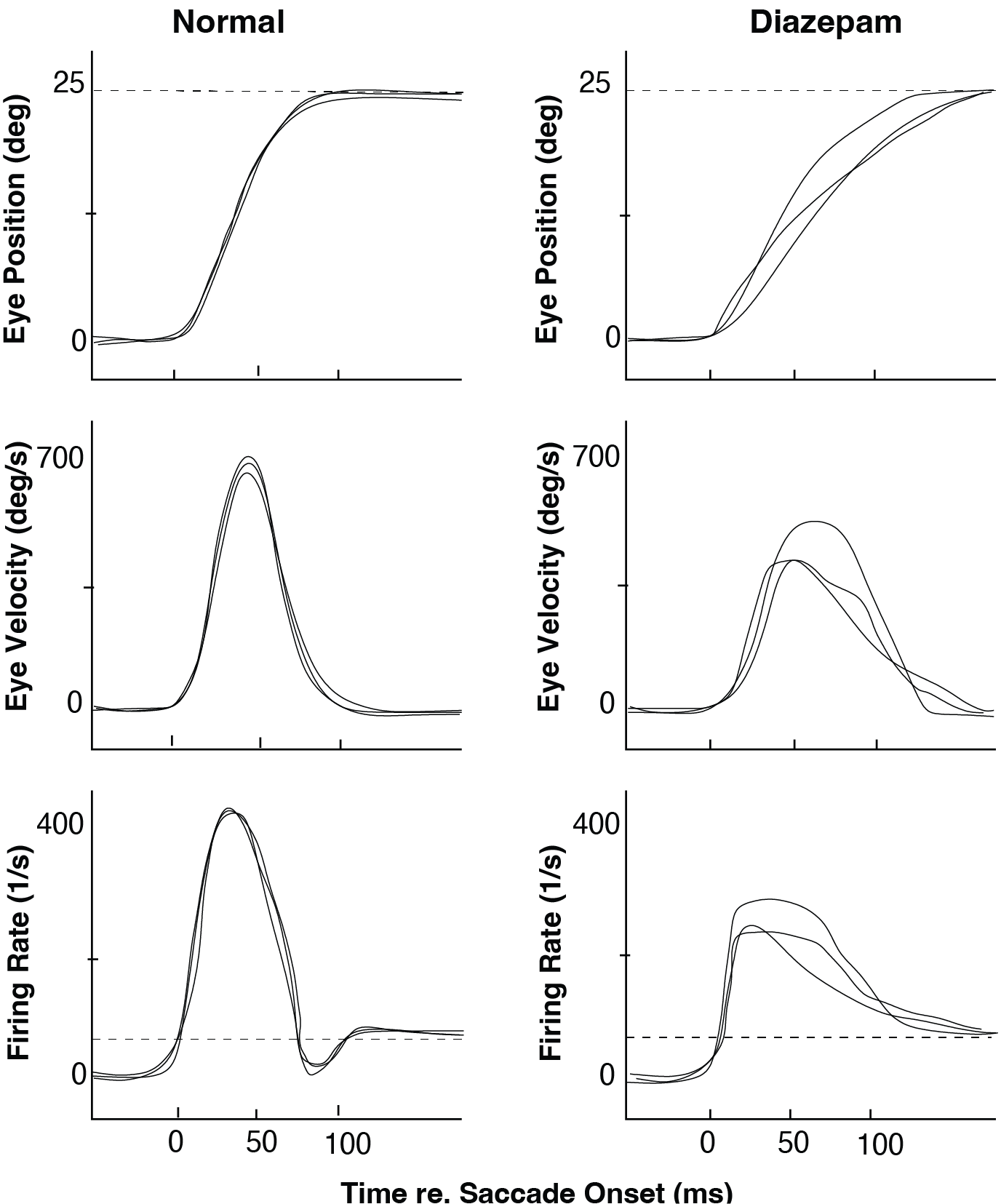
../_images/diazepam.png — Fig. 76 Effect of an intravenous injection of Diazepam (Valium) on human saccades toward flashed targets: although the Valium saccades (right) are still quite accurate, their kinematics are much more variable and slower than normal responses (left). Note also the differences in the reconstructed Pulse-Step signals (bottom). (After: Van Opstal et al., Vision Res., 1985)#

In this exercise, you will try to explain these average experimental findings using the saccade.slx model, under the assumption that:

Valium affects only the CNS (SC, burst generator, feedback, OPNs, etc.),
and does not change the mechanical properties of the oculomotor plant.

That is, keep the Oculomotor Plant parameters (T1, T2) fixed.

Tasks#

Start from the default parameter set of saccade.slx
(use saccade_set_default_params, see Table Table 1).
First create a control condition:
- Adjust the Synaptic Gain so that the model produces a 20° saccade with:
  - a typical, “normal” peak velocity,
  - a typical duration.
- Save these traces (eye position, eye velocity, and (reconstructed) pulse–step command) as the Control condition.
Next, create a “Valium” condition, in which only CNS parameters are changed. For example, you can:
- reduce the Burst Generator saturation level Bmax,
- increase the angular constant Ao (making the burst less sharply accelerating),
- and/or slightly reduce the feedback gain in the brainstem loop.
Keep the Oculomotor Plant (T1, T2) unchanged.

Adjust the Synaptic Gain such that the Valium saccades are still ≈20°, but:
- have lower peak velocities,
- have longer durations, and
- show more trial-to-trial variability (e.g. by adding noise to SC or Synaptic Gain).
Compare:
- eye position and velocity traces (Control vs Valium),
- reconstructed Pulse–Step signals (Control vs Valium).
Explain your findings:
- Which CNS parameters did you change to mimic the effects of Valium?
- Why do these changes slow the saccades but keep their endpoints approximately accurate?
- How do these changes relate to the interpretation that benzodiazepines enhance inhibition and reduce central excitability (without affecting the plant)?

MATLAB Code

%% Exercise 14 — Valium (Diazepam) effects on saccades
% Compare:
%   - Control condition: normal CNS parameters
%   - "Valium" condition: reduced central excitability (CNS only),
%     unchanged oculomotor plant (T1, T2).

disp('Exercise 14 — Valium: CNS changes with fixed plant');

modelName = "saccade";

% -------------------------------------------------------------
% 1. CONTROL: default CNS parameters, calibrate ~20 deg saccade
% --------------------------------------------------------------
saccade_set_default_params(modelName);

% Make sure Burst Generator and Feedback Path are at default
set_param(modelName + "/Burst Generator", ...
    "Bmax", "700", ...   % deg/s
    "Ao",   "7");        % unit of error

set_param(modelName + "/Feedback", ...
    "Gain", "1.0");

% Ensure plant is at default (we will keep this fixed for Valium)
set_param(modelName + "/Oculomotor Plant", ...
    "T1", "0.15", ...
    "T2", "0.020");

% Initial guess for Synaptic Gain
SG0 = 0.5;
set_param(modelName + "/Synaptic Gain", "Gain", num2str(SG0));

% Run once
simOut = sim(modelName);
t = simOut.tout;
y = simOut.yout;

EyePos = y(:,1);
EyeVel = y(:,2);

Amp0   = EyePos(end) - EyePos(1);
Vpeak0 = max(EyeVel);

targetAmp = 20;   % desired amplitude (deg)

% Calibrate Synaptic Gain to get ~20 deg
scaleSG = targetAmp / Amp0;
SG_ctrl = SG0 * scaleSG;
set_param(modelName + "/Synaptic Gain", "Gain", num2str(SG_ctrl));

% Run CONTROL condition
simOut = sim(modelName);
t_ctrl = simOut.tout;
y_ctrl = simOut.yout;

EyePos_ctrl = y_ctrl(:,1);
EyeVel_ctrl = y_ctrl(:,2);

% If you have a Pulse–Step output, set its index here:
% e.g., reconstructed pulse–step might be y(:,3) or y(:,4)
Pulse_ctrl = y_ctrl(:,3);  % <-- adjust to your model

Amp_ctrl   = EyePos_ctrl(end) - EyePos_ctrl(1);
Vpeak_ctrl = max(EyeVel_ctrl);

fprintf('CONTROL: SG=%.3f -> Amp ≈ %.2f deg, Vpeak ≈ %.1f deg/s\n', ...
    SG_ctrl, Amp_ctrl, Vpeak_ctrl);

% -------------------------------------------------------------
% 2. VALIUM: reduced central excitability, fixed plant
% --------------------------------------------------------------
% CNS changes only:
Bmax_val = 350;   % lower saturation velocity
Ao_val   = 14;    % broader, less sharply accelerating burst
K_val    = 0.7;   % slightly reduced feedback gain

set_param(modelName + "/Burst Generator", ...
    "Bmax", num2str(Bmax_val), ...
    "Ao",   num2str(Ao_val));

set_param(modelName + "/Feedback", ...
    "Gain", num2str(K_val));

% Keep plant EXACTLY as in control (no effect on mechanical properties)
set_param(modelName + "/Oculomotor Plant", ...
    "T1", "0.15", ...
    "T2", "0.020");

% We now adjust Synaptic Gain so that Valium saccades are still ≈20 deg
SG_val0 = SG_ctrl;   % start from control gain

set_param(modelName + "/Synaptic Gain", "Gain", num2str(SG_val0));
simOut = sim(modelName);
t_val = simOut.tout;
y_val = simOut.yout;

EyePos_val = y_val(:,1);
EyeVel_val = y_val(:,2);

Amp_val0   = EyePos_val(end) - EyePos_val(1);
Vpeak_val0 = max(EyeVel_val);

scaleSG_val = targetAmp / Amp_val0;
SG_val      = SG_val0 * scaleSG_val;
set_param(modelName + "/Synaptic Gain", "Gain", num2str(SG_val));

% Run VALIUM condition (single trial, mean behaviour)
simOut = sim(modelName);
t_val = simOut.tout;
y_val = simOut.yout;

EyePos_val = y_val(:,1);
EyeVel_val = y_val(:,2);
Pulse_val  = y_val(:,3);   % adjust index if needed

Amp_val   = EyePos_val(end) - EyePos_val(1);
Vpeak_val = max(EyeVel_val);

fprintf('VALIUM (mean): SG=%.3f, Bmax=%.0f, Ao=%.1f, K=%.1f -> Amp ≈ %.2f deg, Vpeak ≈ %.1f deg/s\n', ...
    SG_val, Bmax_val, Ao_val, K_val, Amp_val, Vpeak_val);

% -------------------------------------------------------------
% 3. Plot Control vs Valium: position, velocity, Pulse–Step
% --------------------------------------------------------------
figure;
subplot(3,1,1);
plot(t_ctrl, EyePos_ctrl, 'b-', 'LineWidth', 1.5); hold on;
plot(t_val,  EyePos_val,  'r--', 'LineWidth', 1.5);
xlabel('Time (s)'); ylabel('Eye position (deg)');
title('Eye position: Control vs Valium (~20° saccades)');
legend({'Control','Valium'}, 'Location','best');
grid on;

subplot(3,1,2);
plot(t_ctrl, EyeVel_ctrl, 'b-', 'LineWidth', 1.5); hold on;
plot(t_val,  EyeVel_val,  'r--', 'LineWidth', 1.5);
xlabel('Time (s)'); ylabel('Eye velocity (deg/s)');
title('Eye velocity: Control vs Valium');
legend({'Control','Valium'}, 'Location','best');
grid on;

subplot(3,1,3);
plot(t_ctrl, Pulse_ctrl, 'b-', 'LineWidth', 1.5); hold on;
plot(t_val,  Pulse_val,  'r--', 'LineWidth', 1.5);
xlabel('Time (s)'); ylabel('Pulse–Step (a.u.)');
title('Reconstructed Pulse–Step: Control vs Valium');
legend({'Control','Valium'}, 'Location','best');
grid on;

% -------------------------------------------------------------
% 4. Variability: multiple trials with noise in Synaptic Gain
% --------------------------------------------------------------
% To mimic increased trial-to-trial variability under Valium, we add
% multiplicative noise to Synaptic Gain across trials.

nTrials = 10;

% --- Control variability (small noise) ---
SG_noise_ctrl = 0.05;  % 5% SD
EyeVel_ctrl_trials = cell(1, nTrials);

for k = 1:nTrials
    SG_trial = SG_ctrl * (1 + SG_noise_ctrl * randn);
    set_param(modelName + "/Synaptic Gain", "Gain", num2str(SG_trial));

    % Use CONTROL CNS parameters
    set_param(modelName + "/Burst Generator", ...
        "Bmax", "700", "Ao", "7");
    set_param(modelName + "/Feedback", ...
        "Gain", "1.0");

    simOut = sim(modelName);
    t_tmp = simOut.tout;
    y_tmp = simOut.yout;

    EyeVel_ctrl_trials{k} = [t_tmp, y_tmp(:,2)]; % time + velocity
end

% --- Valium variability (larger noise) ---
SG_noise_val = 0.15;   % 15% SD (more central variability)
EyeVel_val_trials = cell(1, nTrials);

for k = 1:nTrials
    SG_trial = SG_val * (1 + SG_noise_val * randn);
    set_param(modelName + "/Synaptic Gain", "Gain", num2str(SG_trial));

    % VALIUM CNS parameters
    set_param(modelName + "/Burst Generator", ...
        "Bmax", num2str(Bmax_val), "Ao", num2str(Ao_val));
    set_param(modelName + "/Feedback", ...
        "Gain", num2str(K_val));

    simOut = sim(modelName);
    t_tmp = simOut.tout;
    y_tmp = simOut.yout;

    EyeVel_val_trials{k} = [t_tmp, y_tmp(:,2)]; % time + velocity
end

% Plot trial-to-trial velocity variability
figure;
subplot(2,1,1);
hold on;
for k = 1:nTrials
    tv = EyeVel_ctrl_trials{k};
    plot(tv(:,1), tv(:,2), 'Color', [0 0 1 0.3]); % semi-transparent blue
end
xlabel('Time (s)'); ylabel('Eye velocity (deg/s)');
title('Control: trial-to-trial variability (velocity)');
grid on;

subplot(2,1,2);
hold on;
for k = 1:nTrials
    tv = EyeVel_val_trials{k};
    plot(tv(:,1), tv(:,2), 'Color', [1 0 0 0.3]); % semi-transparent red
end
xlabel('Time (s)'); ylabel('Eye velocity (deg/s)');
title('Valium: increased trial-to-trial variability (velocity)');
grid on;

Assignment: The Nonlinear Burst Generator

Contents

Assignment: The Nonlinear Burst Generator#

Learning Goals#

Data#

Downloads#

Research Data Management#

Working With Simulink#

Opening the Model#

Running Simulations#

Viewing Signals#

Editing Parameters#

Creating a Figure#

MATLAB#

Computer exercises with the nonlinear Burst generator model#

Exercise 8 — Pulse–Step Reconstruction#

Task#

Exercise 9 - amplitude#

Exercise 10 — Main Sequence#

Exercise 11 — Influence of the Feedback Gain#

Exercise 12 — Influence of OPN Timing#

Exercise 13 — Superior Colliculus burst#

Part A — Constant number of spikes#

Part B — Changing the total number of spikes#

Exercise 14 — Effect of Valium on Saccades#

Tasks#