The Neural Code

The Neural Code#

learning goals

After studying this chapter, you should be able to:

Explain how neurons encode and decode information.
Describe how spikes are generated and how their frequency and timing carry information.
Distinguish between different coding strategies: rate coding, temporal coding, and labeled-line coding.
List the various types of neural codes, and give specific examples.
Explain the differences between tonic and phasic firing rates.
Describe the stochastic nature of firing rates, in relation to Poisson distributions.
Interpret spike trains using concepts from probability and point-process theory.
Explain how stochastic fluctuations and noise can both limit and improve information transmission.
Compute and interpret interspike interval distributions, and distinguish Poisson, gamma, and refractory-limited spike trains.

Optional Material

Some sections of this chapter include dropdown boxes and downloadable MATLAB code.
These are optional and meant for students who want to explore the material in more depth.
You do not need to study these parts to understand the core concepts.

Introduction#

Neurons communicate using tiny electrical pulses called action potentials, or spikes. You can think of these as the brain’s version of Morse code: brief bursts of electricity that carry information from one neuron to the next. Each neuron receives signals, converts them into its own pattern of spikes, and passes those spikes along to others. Instead of sending smooth, continuous voltages, the nervous system works with discrete events in time: spikes that occur at specific moments. The precise timing and frequency of these spikes form patterns that make up the neural code. In this module, we’ll explore how physical stimuli are encoded into these spike patterns, and how other neurons decode them to make sense of the world.

Encoding and Decoding in the Nervous System#

Neurons communicate by converting sensory input or synaptic activity into patterns of spikes, a process known as encoding. The timing and number of these spikes form a spike train that carries information forward through the nervous system. Downstream neurons then decode these spike trains by integrating incoming spikes over time and across inputs, transforming them back into graded changes in membrane potential that drive further responses. In this way, encoding turns the world into spikes, and decoding turns spikes back into meaningful signals for perception, decision-making, and action.

Although the basic idea is simple—spikes represent information, and other neurons interpret these spikes—the biological details can be rich and varied. Encoding can emphasize firing rates or precise timing, while decoding involves synaptic filtering, temporal integration, and combining information across many neurons.

More about encoding and decoding

Encoding can take many forms depending on the cell type and the sensory system. Some neurons act as feature detectors, responding preferentially to specific stimulus attributes such as motion direction or orientation. Others participate in population codes, where a group of neurons collectively represents a variable such as eye position, sound location, or movement intention.
Decoding within the brain relies on several mechanisms: short-term synaptic dynamics that emphasize or suppress recent spikes, dendritic nonlinearities that amplify specific patterns, and recurrent network activity that integrates information across time and space. These same principles are used by researchers when decoding neural signals experimentally, whether from single-unit recordings, multi-electrode arrays, calcium imaging, or Neuropixels probes.

Sensory Coding: How Senses Transmit Information#

Sensory signals vary in many ways: they have a modality (light, sound, touch), a quality (color, pitch, location), a quantity or intensity, and a temporal structure. The nervous system must therefore transform each stimulus into a spike pattern that preserves these different aspects while remaining compatible with the brain’s spike-based communication system.

To accomplish this, sensory systems use several coding strategies. For distinguishing what kind of stimulus has occurred—whether something is visual, auditory, or tactile—the nervous system relies on specialized pathways. Each sensory modality is carried by its own dedicated nerves and brain areas, forming the foundation for the labeled line principle described below.

Within each sensory pathway, neurons must also encode properties such as stimulus intensity, timing, and fine structure. This can be achieved by changing the number of spikes (rate coding), the timing of spikes (temporal coding), or by combining activity across many neurons (population coding). These codes allow the brain to represent both slow changes, such as brightness or loudness, and fast fluctuations, such as vibration or temporal modulations in sound.

In the next section, we explore the Labeled Line Code, which ensures that different types of sensory signals remain separated. After that, we will examine how the pattern of spikes—their count and timing—represents the quantity and temporal structure of the sensory input.

Key aspects of sensory coding

Modality: This refers to the type of stimulus, such as light, sound, temperature, or chemical composition (like salt concentration). Different sensory modalities are processed by specific sensory systems in the body.
Quality: Within each modality, there are subtypes or qualities of stimuli. For instance, in the modality of vision, different colors are perceived; in taste, various flavors are distinguished.
Quantity: This aspect covers the intensity or strength of a stimulus. It could be the brightness of light, the loudness of sound, or the concentration of a substance.
Temporal Structure: This involves the timing aspects of a stimulus, like the rhythm of a sound or the pattern of light pulses.
Stochastics: This refers to the random elements inherent in sensory processing. These can sometimes negatively impact signal clarity but can also enhance signal detection under certain conditions.

The Labeled Line Code#

For coding two aspects of sensation—modality (the type of stimulus) and quality (its subtype)—the nervous system often uses a labeled line code. This means that specific nerve pathways are dedicated to carrying specific kinds of sensory information. For example, olfactory signals travel via the first cranial nerve, while visual signals are transmitted through the second cranial nerve. Within each sensory system, further specialization occurs: different nerve fibers can respond to different colors in vision, frequencies in hearing, or locations on the skin.

doctrine of specific nerve energies

An important idea related to this is the Doctrine of Specific Nerve Energies, first proposed by Johannes Müller in the 19th century. It states that the sensation we experience depends not on the physical nature of the stimulus itself, but on which nerve is activated. In other words, it is the pathway, not the energy, that determines the kind of perception.

A simple and striking example is what happens if you gently press on your closed eyeball: you will “see” flashes of light or moving patterns, known as phosphenes. No light actually enters the eye—the mechanical pressure merely excites the optic nerve. Because that nerve normally carries visual information, the brain interprets this activity as seeing light. This illustrates how each sensory system has its own labeled channel: stimulation of the optic nerve—by light, pressure, or electricity—always leads to a visual experience.

sensory prostheses

The same principle underlies modern sensory implants. Electrical stimulation of a sensory nerve or brain area can evoke the same kind of perception as a natural stimulus, because the brain interprets activity in a nerve by its origin, not by its cause.

For example, in a cochlear implant, tiny electrodes inserted into the cochlea directly stimulate auditory nerve fibers. Even though the ear’s hair cells are bypassed, activation of these auditory pathways still produces the sensation of hearing. By varying which electrodes are activated, the implant can convey information about sound frequency replacing the natural labeled lines of the auditory system.

Similar approaches are used in retinal and visual cortex implants, where patterned electrical stimulation of visual pathways can create the perception of light spots or simple shapes.

In each case, the quality of the sensation—hearing or seeing—depends entirely on which neurons are stimulated, not on the physical form of the stimulus.

Although the labeled line code explains how different sensory modalities and qualities are kept distinct, it does not tell us how much of a stimulus is present or when it occurs. For example, within a single labeled line—say, an auditory nerve fiber—the loudness of a sound or the timing of a modulation must still be represented in the pattern of spikes it produces. In the remainder of this chapter, we will not further discuss labeled lines, but instead focus on how spike trains encode these dynamic aspects of neural signaling. We will look at rate coding, where information is carried by the number or frequency of spikes, and temporal coding, where the exact timing of spikes conveys crucial details about the stimulus. Together, these coding strategies reveal how neurons transform continuous physical events into discrete electrical messages that the brain can interpret.

The Spike Code#

In contrast to the labeled line code — which specifies which sensory pathway is active — neurons also use spike-based codes to represent the properties of a sensory signal. These spike codes come in two complementary forms: rate coding and temporal coding. Both arise directly from the biophysics of action-potential generation. When a neuron receives stronger or more sustained input, it reaches threshold more quickly and more often, producing a higher spike frequency — the essence of a rate code. At the same time, the mechanisms that govern spike initiation determine exactly when spikes occur, allowing precise timing of spikes to represent rapid changes, rhythms, or fine temporal features of the stimulus. In the next sections, we will see how these changes in spike frequency and spike timing emerge and how they allow neurons to encode both the intensity and the temporal structure of sensory input.

Rate Code#

The Single Spike: Action Potential#

Neurons generate action potentials when their membrane potential becomes sufficiently depolarized to reach a threshold. At rest, the membrane sits at a stable negative potential. When excitatory input arrives — through synaptic currents or sensory transduction — it pushes the membrane potential upward. If this depolarization crosses threshold, voltage-gated ion channels open and an action potential is initiated (Fig. 21).

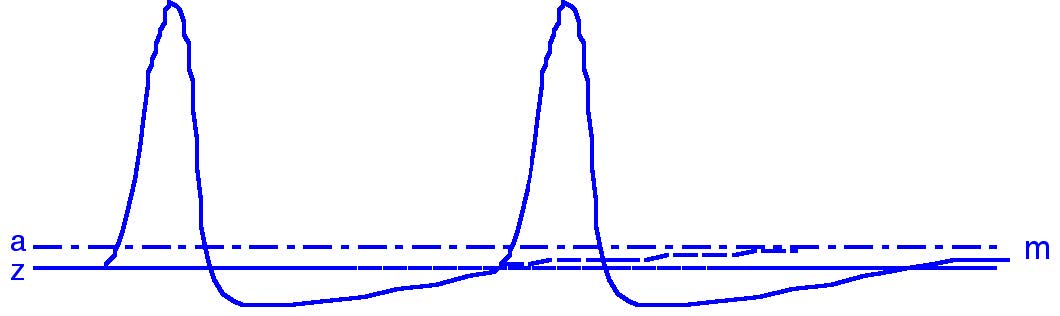
../_images/figure1.jpg — Fig. 21 Threshold for the generation of action potentials. The thick line (m) shows the membrane potential; the threshold level (z) indicates when a spike is generated.#

The distance between the resting potential and the threshold determines how easily a neuron can fire.

Neurons with thresholds close to rest may fire spontaneously due to small fluctuations.
Neurons with thresholds far from rest (e.g., many mechanoreceptors) require stronger stimulation.

After every spike, the membrane briefly becomes hyperpolarised, creating a refractory period during which another spike cannot occur. This sets a minimum time between spikes and ensures spikes remain discrete events.

Spike Trains#

A single spike is just one event, but a neuron usually fires sequences of spikes when stimulated. These sequences — spike trains — are the basis of spike-based neural coding. Although real action potentials have finite width, we can mathematically describe a spike train by marking when each spike occurs:

(17)#\[\rho(t) = \sum_{i=1}^n \delta(t-t_i)\]

Here, \(\rho(t)\) is the neural response function, and each \(\delta(t - t_i)\) is a Dirac pulse indicating a spike at time \(t_i\). This idealization lets us treat spikes as timed events, which will be crucial for understanding both rate and temporal codes.

From the Signals chapter, recall that a delta function can reconstruct any signal:

(18)#\[ \int_{-\infty}^{+\infty} x(\tau) \cdot \delta (t-\tau) d\tau = x(t)\]

In the same spirit, we can think of a neuron as representing a stimulus through the timing and number of spikes it generates. To understand what a spike train represents — how the signal is decoded — we must determine how much each spike contributes to downstream activity.

Firing Rate#

Changes in membrane potential caused by sensory input directly influence how often a neuron reaches threshold. Stronger depolarizing input makes the membrane climb toward threshold more quickly after each spike, producing a higher firing rate. Weaker input slows this recovery, lowering the rate. Thus, spike frequency naturally reflects the intensity of the driving stimulus.

Empirical recordings, such as those from stretch receptors (Fig. 22a), show that firing rate often increases monotonically with stimulus strength, making rate a robust code for “how much” stimulus is present. However, the threshold is not fixed (Fig. 22b,c). During the refractory period, excitability is reduced, and even after recovery, many neurons show adaptation: firing rate declines over time despite a constant stimulus. This produces two characteristic response types:

Tonic receptors (Fig. 22a,b): Fire throughout the stimulus with mild adaptation (slowly adapting).
Phasic receptors (Fig. 22a,c): Respond strongly at onset but adapt quickly (rapidly adapting).

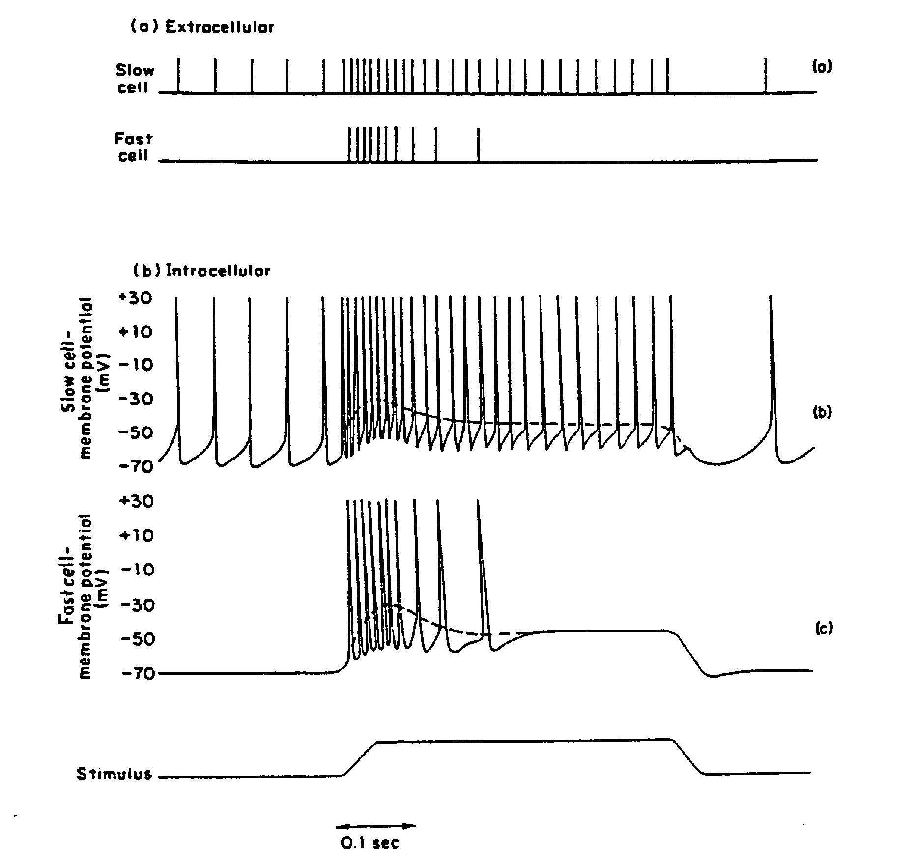
../_images/figure3.jpg — Fig. 22 Difference between tonic (‘slow’; top) and phasic (‘fast’; bottom) response of a sense cell or nerve cell, as expressed in extracellular (a) and intracellular (b, c) measurements. The difference does not (always) appear to be in the course of the membrane potential, but is a property of the spike generation mechanism. Taken from Gordon et al. (1977).#

Tonic and phasic components can also coexist within a single neuron. A classic example comes from the oculomotor system, where motor neurons that control eye movements show a combined pulse–step pattern of activity (Fig. 23). These neurons fire at a steady tonic baseline rate during fixation. When a rapid eye movement (a saccade) is initiated, they produce a brief, high-frequency phasic burst — the pulse — to drive the eye quickly to a new position. After the movement, their firing settles into a new tonic level — the step — that is higher than baseline and maintains the eye in its eccentric position. This example illustrates how a single neuron can multiplex both phasic and tonic firing to encode different aspects of a motor command.

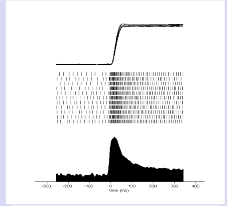
../_images/oculomotor_pulse_step.png — Fig. 23 Oculomotor neurons combine tonic and phasic firing. A high-frequency phasic “pulse” drives a rapid eye movement, while the tonic “step” maintains the new eye position.#

In some neurons, pacemaker currents introduce slow oscillations that cause spikes to appear in bursts rather than evenly spaced. Even in these cases, the average firing rate over time can still carry meaningful information.

Encoding quantity#

The strength or quantity of a stimulus can be represented directly in the firing rate of a single neuron. As input becomes stronger — whether a louder sound, a brighter light, or greater muscle stretch — the neuron depolarizes more rapidly, reaches threshold sooner after each spike, and therefore fires at a higher rate (Fig. 24, top). This simple relationship forms the basis of the rate code for stimulus intensity.

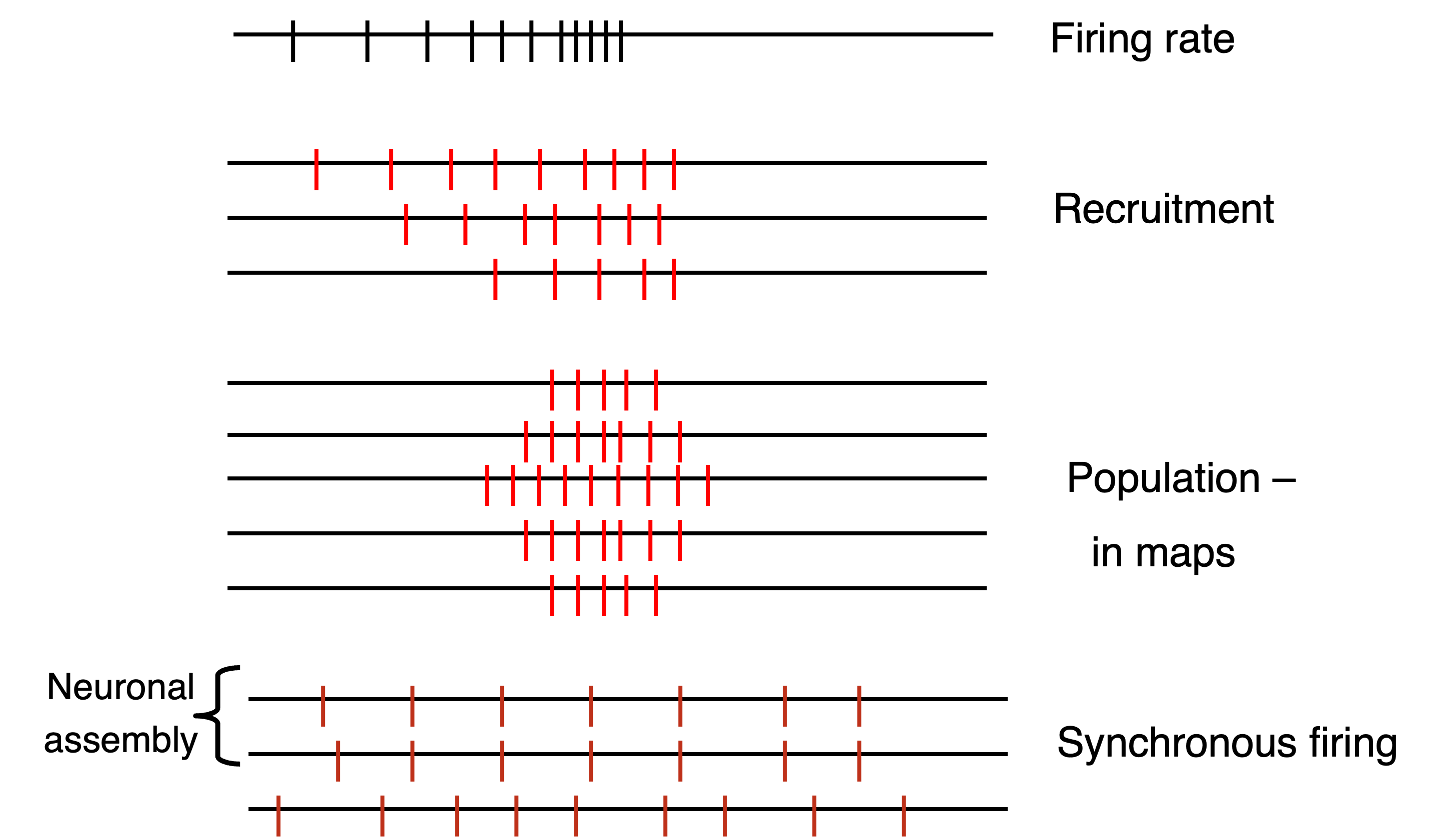
../_images/neuralcodes.png — Fig. 24 Encoding of quantity by firing rate.#

However, many sensory and motor systems operate over a large dynamic range, far broader than a single neuron can represent on its own. To extend this range, the nervous system uses recruitment (Fig. 24, 2nd row): as stimulus strength increases, more neurons begin to respond. For example, in the auditory nerve, low sound levels activate only the most sensitive fibers, while higher levels recruit additional fibers with higher thresholds. Similarly, in the oculomotor system, neurons increase their firing rate with eye position, but different neurons cover different parts of the range, together encoding the full span of possible gaze angles.

A related strategy is population coding (Fig. 24, 3rd row), where a group of neurons jointly represents stimulus strength. In this scheme, the pattern of activity across many neurons conveys the quantity more robustly than any single neuron alone. A well-known example comes from the superior colliculus, where neurons have “movement fields”: each neuron fires most strongly for saccades of a particular size and direction, but many neurons contribute to encoding the exact amplitude of the movement. The brain interprets the overall population response to determine the stimulus magnitude or motor command.

Together, recruitment and population coding allow the nervous system to encode stimulus strength with high resolution, wide dynamic range, and robustness to noise, far beyond what any single neuron could achieve.

Spike Timing#

Stochasticity#

Even when a neuron is stimulated in exactly the same way, its spike train will not be identical from trial to trial. Small fluctuations in ion channels, synaptic release, and membrane potential introduce stochasticity — random variability in when spikes occur. This raises an important question: if a neuron fires slightly faster in one moment (Fig. 25), is that because the stimulus became stronger, or simply because of chance?

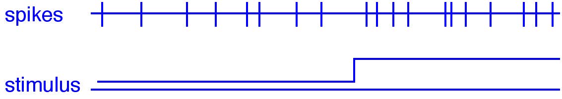
../_images/figure5.jpg — Fig. 25 Stochastic fluctuations in a spike train. The bottom trace shows a stimulus that becomes stronger halfway through.#

Because spikes are discrete events that occur at particular times, spike trains are naturally described using point process theory. When recording extracellularly, we typically extract only the times of the spikes (not their shapes), because the exact waveform carries little information. Thus, a spike train from a single neuron can be viewed as a one-dimensional point process — a set of event times scattered along the time axis.

Stochasticity does not mean “meaningless noise.” Instead, it means that we — and the central nervous system — must interpret spike trains statistically, taking into account variability and probability rather than relying on exact timing alone, to arrive at a reliable interpretation of the input signal.

Poisson Process#

The variability (“stochasticity”) we observe in spike timing can be described mathematically using point-process models. One of the most important of these is the Poisson process, which provides a simple statistical description of how spikes might occur when each spike is generated independently and with some underlying probability per unit time. We therefore introduce the Poisson process as a basic model for understanding the irregularity seen in neural spike trains. In a Poisson process, spikes occur:

independently of previous spikes
with a constant probability per unit time
and with a single governing parameter, the mean firing rate \(\lambda\) (spikes/s)

Because each spike is independent, the process is said to be memoryless. Knowing when the last spike occurred provides no information about when the next one will happen.

memoryless

It may seem surprising that neurons—biological systems with membrane capacitance, ion-channel kinetics, and synaptic dynamics—could approximate such a memoryless process. Each of these mechanisms indeed introduces temporal structure. But an action potential itself is a biophysical reset: when thousands of voltage-gated sodium and potassium channels open and close during a spike, the membrane is driven into a stereotyped state. After the refractory period, the neuron effectively “forgets” the exact conditions of the previous spike, making successive intervals approximately independent. This is why the spontaneous activity of many sensory neurons resembles a stationary Poisson process with a constant mean rate.

Many real-world phenomena behave this way. A classic example is the failure of light bulbs: if the average lifespan of a bulb is 1000 hours, you know the mean behavior, but not when your bulb will fail. A brand-new bulb may burn out within an hour, while another lasts 2000 hours. The probability of failure is independent of how long the bulb has already been operating—exactly the “memoryless” property of a Poisson process. Similar behavior occurs for cars passing a point on a highway, radioactive decay, and many other systems.

A useful way to visualize Poisson behavior is to count the number of spikes in a fixed time window (Fig. 26). If spikes occur as a Poisson process with mean rate \(\lambda\), then the number of spikes \(k\) observed in a window of duration \(T\) follows the Poisson distribution with mean \(\mu = \lambda\) and standard deviation \(\sigma = \sqrt{\lambda}\):

\[p(k \mid \lambda) = \frac{\lambda^k}{k!} e^{-\lambda}.\]

At low mean rates, this distribution is strongly skewed (Fig. 26). At higher mean rates, it becomes more symmetric and approaches a Gaussian distribution due to the central limit theorem.

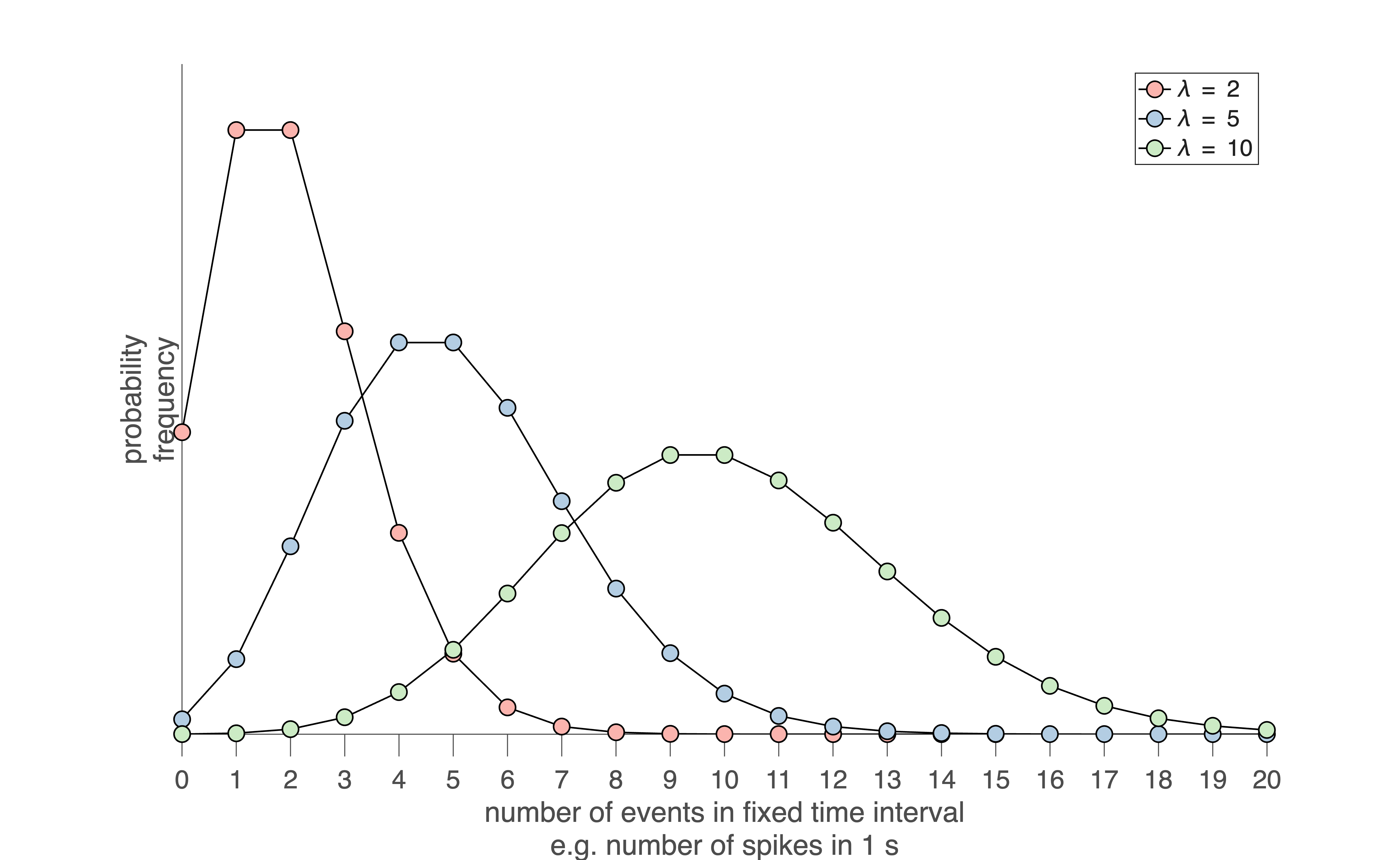
../_images/spike_poisson_pdf.png — Fig. 26 | Poisson distribution.#

Three Poisson probability distributions for spike counts measured in a fixed time window (e.g., number of spikes occurring in 1 second). When the mean count \(\lambda\) is small, the distribution is highly skewed toward zero. As \(\lambda\) increases, the distribution becomes broader and more symmetric, eventually approaching a Gaussian shape due to the central limit theorem. `Download Matlab code to generate this figure`

Spike interval distribution#

Counting spikes is only one way to analyze variability. Equally important is examining how much time separates one spike from the next — the interspike interval (ISI). (We ignore the brief duration of the spike itself; it carries no information.) If every interval is identical, the spike train is regular, like the perfectly periodic ticking of a clock — predictable and low in information. Real neurons almost never behave this way. Instead, their intervals vary from spike to spike, producing irregular firing patterns, and this irregularity may be informative.

ISI ~ exponential distribution#

If spikes occur according to a Poisson process, then the ISIs follow an exponential distribution:

very short intervals are most probable
long intervals become progressively less likely
the process has no memory: knowing when the last spike occurred does not change the probability of the next one

This exponential ISI distribution is shown in Fig. 27A.

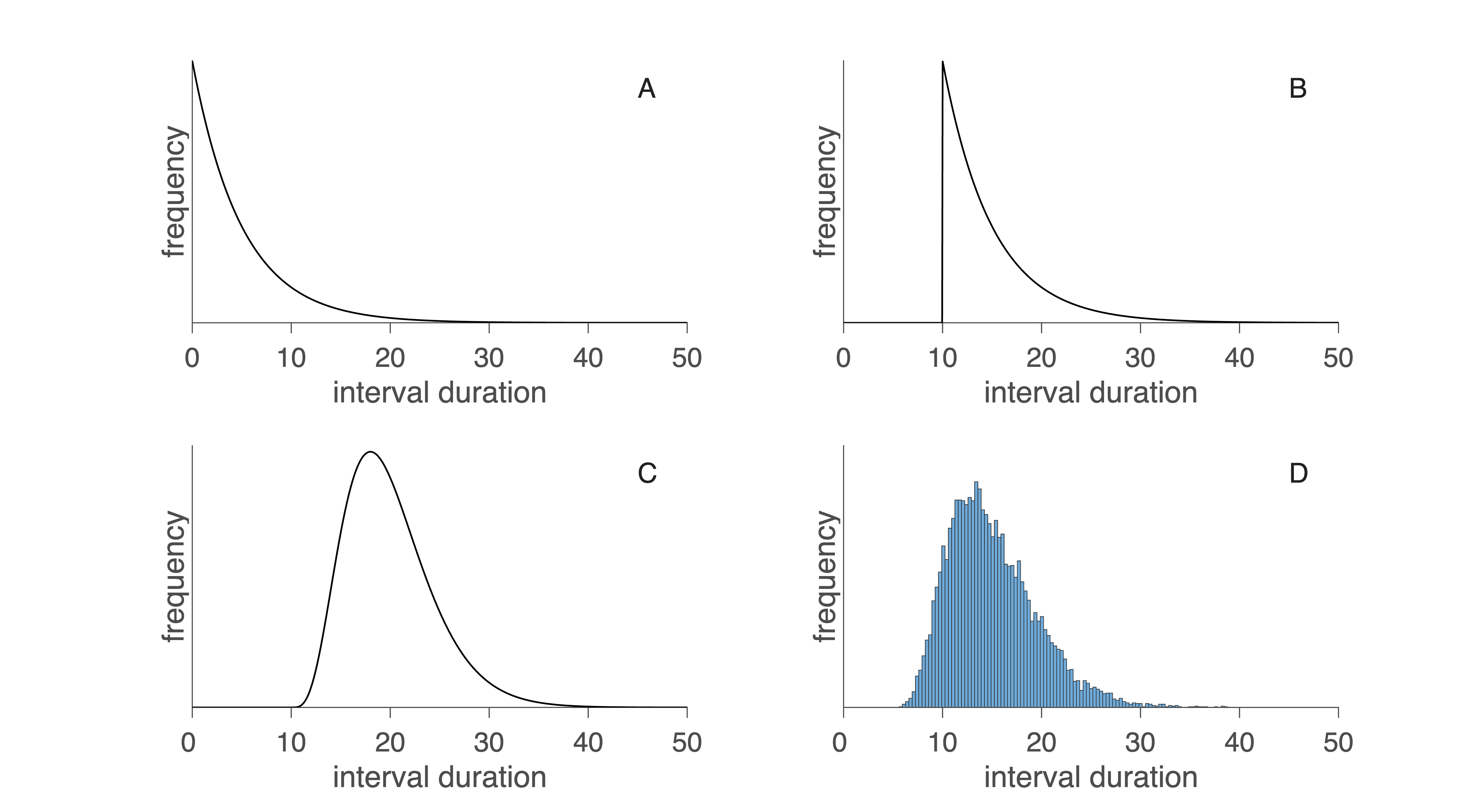
../_images/spike_isi_distribution.png — Fig. 27 Interspike interval distributions. A: exponential distribution of intervals at pure Poisson-distributed events. B: the same, now taking into account the refractory time. C: gamma distribution for the sum of a number of events. D: Practical example of an interval histogram. `Download Matlab code to generate this figure`#

Refractory period#

Real neurons cannot fire arbitrarily fast. After each action potential, there is a brief refractory period during which no new spike can occur. This creates a short dead time in the ISI distribution (Fig. 27B), eliminating the shortest possible intervals and shifting the distribution slightly to the right.

Gamma distribution#

Many neurons deviate from this simple Poisson-with-dead-time model. Two main factors cause more complex ISI distribution shapes:

Dependence between intervals. Adaptation, bursting, or rhythmic oscillations introduce correlations across intervals.
Multiple small events required for a spike. At some synapses, individual vesicle releases are insufficient; several must summate to reach threshold. In this case the ISIs follow a gamma distribution (Fig. 27C), which has:

few very short intervals
a peak at intermediate intervals
variability governed by how many events must accumulate

When many such small events are required (e.g., many small depolarizations must summate before firing), the ISI distribution becomes increasingly Gaussian due to the central limit theorem. Real neurons therefore show diverse ISI patterns (Fig. 27D), revealing much about the underlying spike-generation mechanism.

Quantifying Spike Train Variability#

Two standard measures capture different aspects of neural variability.

1. Fano factor (spike count variability)#

For a Poisson process, spike counts in a fixed time window have equal mean and variance. The Fano factor measures this:

\[F=\frac{\sigma^2}{\mu}\]

\(F = 1\): consistent with Poisson count statistics
\(F < 1\): more regular than Poisson
\(F > 1\): more variable (bursting, modulation, heterogeneity)

Care must be taken to analyze spontaneous and stimulus-driven spikes separately because stimulation typically changes the mean rate, which affects the Fano factor. A disadvantage of the Fano factor is that it is not dimensionless (so, it depends on the units in which the measurement is taken, e.g. ms vs. s). Another measure, which is dimensionless, is the Coefficient of Variation.

2. Coefficient of Variation (ISI variability)#

The coefficient of variation (CV) quantifies the variability of interspike intervals:

\[CV = \frac{\sigma}{\mu}\]

For exponential ISIs (i.e., Poisson timing), \(CV = 1\). Values:

\(CV < 1\): more regular firing (clock-like)
\(CV > 1\): irregular or bursty firing

Using Fano Factor and CV Together#

Both the Fano factor and the coefficient of variation (CV) quantify variability, but they do so in different ways:

The Fano factor compares variance to the mean: \(F = \frac{\sigma^2}{\mu}\)
The CV compares standard deviation to the mean: \(CV = \frac{\sigma}{\mu}\)

Because they normalize variability differently, they capture different statistical properties of a spike train.

For a true Poisson point process:

Spike counts follow a Poisson distribution: variance = mean → Fano factor = 1
Interspike intervals follow an exponential distribution: standard deviation = mean → CV = 1

Thus:

Fano factor = 1 is the signature of Poisson count statistics
CV = 1 is the signature of Poisson interval statistics

Because the two metrics capture different aspects of variability, using both together provides a clearer picture of whether spiking behaves like a Poisson process or whether additional mechanisms—refractoriness, adaptation, bursting, or synaptic summation—shape the spike train.

Noise#

So far, we have seen that neural activity contains substantial variability: spike times jitter, firing rates fluctuate, and responses differ from trial to trial. In everyday language this variability is called noise, but in neuroscience that term can be misleading. There are two fundamentally different reasons why neural signals appear noisy, and they have very different implications.

1 - Apparent noise#

The variability we see may actually be deterministic, but we are just not measuring everything. Sometimes a spike train looks random simply because we can only observe a small part of a complex system. A classic example comes from Bullock (1970): recording a single cortical neuron is like monitoring the “E” key inside the Pentagon’s typewriter room. Its activity looks chaotic, but the larger system — the entire text being written — is completely orderly. A modern analogy: tapping into one line of a computer’s data bus would show rapid, seemingly random 0s and 1s. But when all eight bits are viewed together, the pattern reveals meaningful characters:

“A” might correspond to 01000001
“a” might correspond to 01100001

If you only look at bit 5, it flips between 0 and 1 in a way that appears random, but actually reflects meaningful structure within the full pattern. Likewise, in neural recordings, fluctuations in a single neuron’s spike train may reflect structure elsewhere in the circuit, not randomness. In that sense, variability is often just unexplained variance, not true noise.

2 - True noise#

There may be true biological randomness, but as we will now see, neural noise can improve signal representation. Neurons also exhibit genuine stochasticity, arising from physical and molecular processes:

Ion channels open and close probabilistically at body temperature (≈300 K).
Synaptic vesicles release neurotransmitter quanta independently.
Membrane potentials fluctuate due to thermal agitation and molecular noise.

This noise is not caused by incomplete measurement; it is an inherent part of neural computation. Importantly, true noise can play two essential roles in neural coding.

2a - Noise improves the rate code#

The apparent contradiction in the title of this section has to do with the neural signals being a repeated series of action potentials - rather than a continuous signal. Noisy fluctuations in the spike trains can have a useful, and even necessary influence on signal representation as we will explain for an auditory nerve fiber. To understand why noise can be useful for representing stimulus strength, consider how an auditory nerve fiber responds to a low-frequency tone. The panels in Fig. 28A and B show spike trains recorded from a fiber stimulated with a tone of about 100 Hz at two different sound levels.

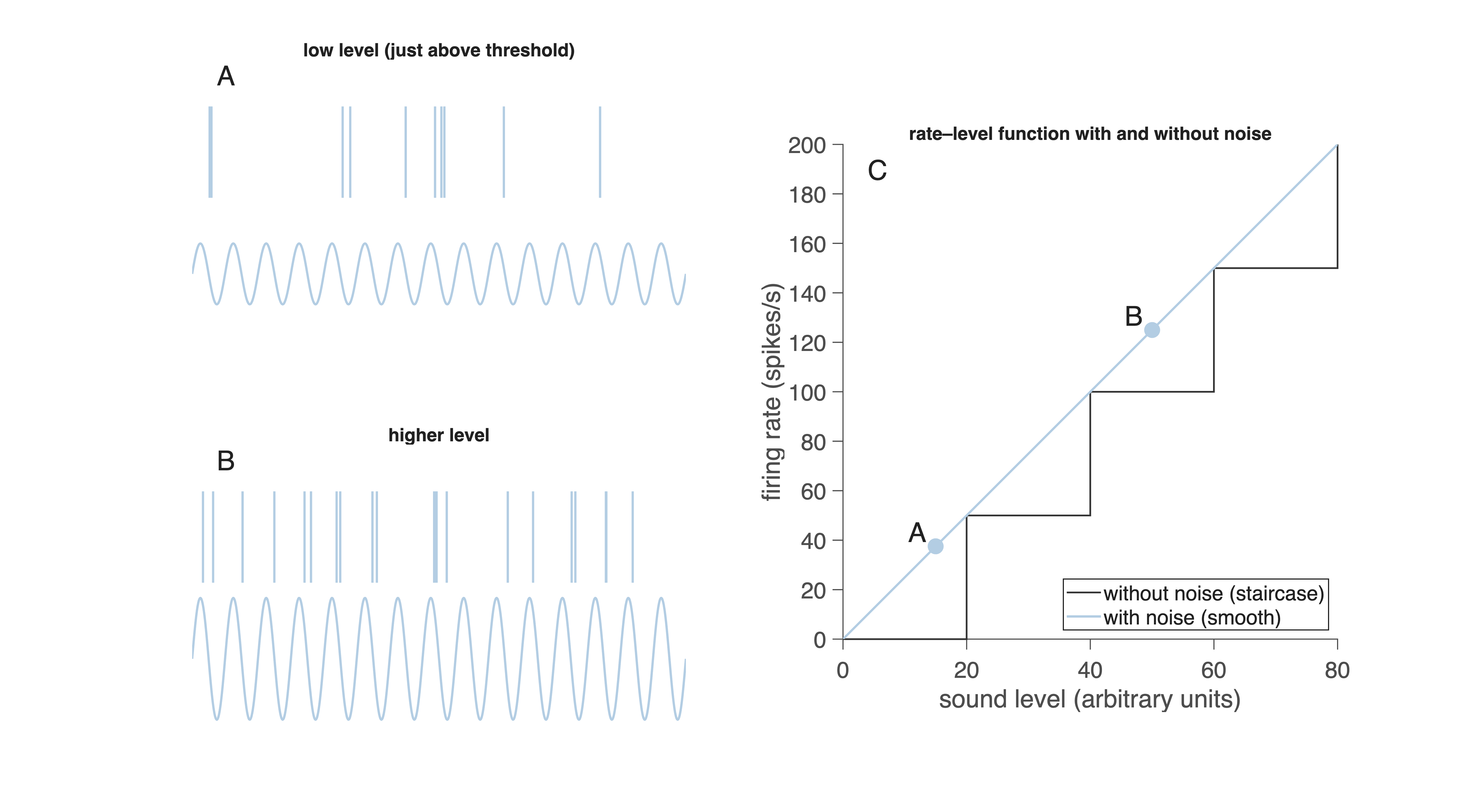
../_images/spike_noise_rate.png — Fig. 28 A, B: Auditory nerve responses to a ~100 Hz tone at two intensities.
C: Without noise, the rate–level function is a staircase; with noise, it becomes smooth and usable. `Download Matlab code to generate this figure`#

In a typical auditory hair cell, each peak of the sound wave depolarizes the receptor potential. That depolarization may or may not be sufficient to trigger one spike in the auditory nerve. Because of biological fluctuations — in synaptic release, ion-channel noise, and membrane potential — each stimulus cycle produces:

sometimes no spike,
sometimes one spike,
sometimes more than one spike.

This variability is visible in Fig. 28A and B. At low sound levels (A), the fiber fires only occasionally. At higher levels (B), spikes occur more often but still not perfectly regularly. At first glance, this looks like a limitation: if one cycle sometimes produces a spike and sometimes does not, how can the brain reliably detect sound level?

To answer this, imagine what would happen if the neuron had no noise at all, and thus produced a fixed number of spikes per stimulus cycle. That situation is shown schematically in Fig. 28C (step-shaped line). In this idealized noiseless system:

below threshold → 0 spikes per cycle
just above threshold → exactly 1 spike per cycle
at higher levels → exactly 2 spikes per cycle
and so on

This results in a staircase-shaped input–output curve: long flat segments (no change in firing rate) punctuated by abrupt jumps when a new integer number of spikes per cycle becomes possible. Such a response cannot convey small changes in sound level—there is no gradual increase in firing rate, only discrete steps. This would create strange and unusable percepts: sound level would seem to change suddenly, with no smooth transitions. Now look at the smooth line in Fig. 28C. This is the curve observed with biological noise. Because each cycle has a probability of producing a spike, the average firing rate increases continuously with sound level. Even a very weak sound produces occasional spikes; stronger sounds produce spikes more often. In Fig. 28A the fiber fires on about 0.38 cycles per period; in Fig. 28B on about 1.25 cycles per period. Noise therefore linearizes the staircase, turning it into a smooth, information-rich function.

This is why noise improves rate coding:

It prevents the response from being locked to rigid, integer-valued spikes per cycle.
It makes the firing rate change smoothly (linearly) with stimulus strength.
It allows the nervous system to encode fine differences in intensity.
It enables probabilistic coding, which downstream neurons can decode by averaging over time (temporal integration) or over many neurons (spatial integration). Thus, noise is not merely a nuisance — it is necessary for creating a useful rate code over a wide dynamic range.

2b - Noise improves the temporal code#

Noise does not only help neurons encode how strong a stimulus is—it can also improve how they encode when things happen. To see this, consider a simulated neuron responding either spontaneously or to a sinusoidal input, with different amounts of noise added. Figure Fig. 29 shows spike trains from a simulated neuron, together with the corresponding peristimulus time histogram (PSTH).

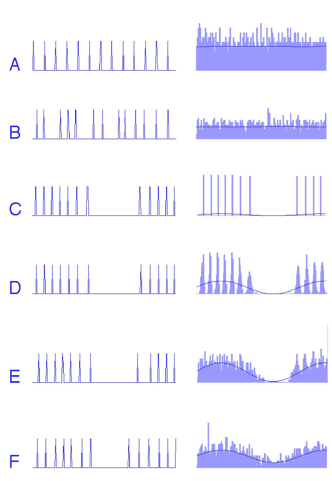
../_images/figure9.jpg — Fig. 29 Effect of noise on temporal coding.
Left column: short segments of simulated spike trains.
Right column: corresponding peristimulus time histograms (PSTHs) with fitted sine waves.
A–B: spontaneous activity with no noise (A) and with noise (B).
C: noise-free neuron responding to a sinusoid (strict phase locking).
D–F: neuron responding to a sinusoid with increasing noise levels (–20 dB, –10 dB, 0 dB). Spike density increasingly follows the sinusoidal stimulus.#

A PSTH is constructed by aligning spikes to repeated cycles of a stimulus — in this case the positive zero-crossing of a sinusoid — and counting how many spikes occur at each moment within a single cycle. It shows the probability of spiking as a function of stimulus phase, compressing many cycles into one representative period.

At first, consider the spontaneous activity of the model neuron without noise (A). The spike train is highly regular, firing almost periodically, and the PSTH remains nearly flat because the spikes are not aligned to any meaningful stimulus phase. When a small amount of noise is added (B), the spike times become slightly more variable, producing a smoother PSTH and avoiding sampling artifacts that occur when a regular spike train is sampled at a similar frequency.

The effect becomes clearer when a sinusoidal input is introduced. Without noise (C), every spike occurs at exactly the same phase of the sinusoid. This perfect phase locking prevents the neuron from representing the shape of the waveform: the PSTH collapses into a sharp peak, and the fitted sine wave does not resemble the true stimulus. The neuron behaves more like a timing device than a waveform encoder.

As noise is added to this sinusoid-driven neuron (D–F), spike timing begins to jitter around the phase-locked point. This jitter spreads spikes across the sinusoidal cycle in proportion to the momentary drive of the stimulus. When these jittered spikes are averaged into a PSTH, the result begins to resemble the actual sinusoidal input more closely. At moderate to high noise levels (F), the PSTH follows the sinusoidal waveform almost perfectly, and the fitted sine wave aligns with the true input.

Thus, noise allows the neuron to represent the temporal structure of the signal by reducing excessive phase locking. A small amount of variability enables spikes to carry information about when the stimulus is high or low, rather than simply firing at one rigid moment each cycle. This effect — often called stochastic resonance — shows that noise can enhance temporal coding, provided that enough cycles (or enough neurons) are averaged together.

Deterministic chaos

3 - Deterministic chaos

There is a third reason why neural signals appear noisy. Some seemingly noisy neural signals may arise from deterministic chaos — complex but deterministic dynamics that are highly sensitive to initial conditions (as seen in weather systems and turbulent flows). In spike trains, chaotic firing produces characteristic patterns in interspike interval dot plots:

True stochastic noise → a diffuse cloud
Deterministic chaos → stripes or structured bands

This reminds us that variability in neural data may arise from multiple sources: limited observations, true biological randomness, or nonlinear deterministic dynamics.

Decoding Spike Trains

Up to now, we have focused mostly on how neurons encode information by converting sensory input into spike trains. But this is only half of the story. For neural signals to have any effect—on perception, decision-making, or movement—they must also be decoded. Decoding refers to the set of processes by which neurons, circuits, and researchers interpret spike trains to recover the information they carry.

Neural decoding within the brain

Postsynaptic neurons decode spike trains by integrating their incoming spikes over time and across inputs. At low firing rates, individual action potentials generate discrete postsynaptic potentials that can still be distinguished from one another. At higher firing rates, these potentials overlap and summate into a smoother depolarization whose magnitude reflects the firing rate of the presynaptic neuron.

Thus, the nervous system continuously extracts information through:

temporal integration: averaging spikes over time, smoothing out variability
spatial integration: pooling across many presynaptic neurons
synaptic filtering: shaping responses with short-term plasticity and receptor kinetics
nonlinear dendritic processing: boosting or suppressing specific spike patterns

In this way, a spike train that appears noisy or irregular at the single-neuron level becomes a stable, interpretable signal at the circuit level.

Decoding by researchers

When we record neural activity, we face a similar challenge: how do we infer what a neuron—or a whole population—is representing?

Neuroscientists decode neural activity using many of the same principles as the brain:

Rate decoding: interpreting information from the average firing rate
Temporal decoding: analyzing spike timing, synchrony, and phase
Population decoding: reconstructing stimuli or behaviors from groups of neurons

Classic single-electrode recordings provided access to one neuron at a time, limiting the kinds of decoding questions researchers could ask. But modern techniques allow us to record tens, hundreds, or even thousands of neurons simultaneously, opening up entirely new forms of decoding analysis.

Modern large-scale recording techniques

Recent technological advances have revolutionized our ability to decode neural activity:

Multi-electrode arrays (MEAs) and Neuropixels probes. Record hundreds to thousands of neurons across multiple brain areas simultaneously, with high temporal precision.
Calcium imaging (1-photon, 2-photon). Measures neural activity indirectly by imaging calcium influx associated with firing. This allows simultaneous recording from large populations—sometimes tens of thousands of neurons—with cellular-level spatial resolution.
Voltage imaging. A newer technique that can track rapid membrane potential changes across populations, approaching the temporal resolution of electrophysiology.
Optogenetic tagging and circuit interrogation. Enables identification of specific cell types or synaptic pathways while recording.

These methods make it possible to investigate population coding, distributed representations, and complex sensory-motor transformations in ways that were impossible a decade ago. With such large datasets, decoding now often involves computational techniques such as:

Bayesian decoding
Generalized linear models (GLMs)
Dimensionality reduction (PCA, t-SNE, UMAP, factor analysis)
Neural manifold analysis
Machine learning classifiers and deep networks

In many cases, population activity reveals structure that is not visible when analyzing single neurons alone.

Decoding closes the loop

Neural encoding describes how the brain transforms the world into spikes. Neural decoding describes how the brain—and researchers—extract meaning from these spikes. Large-scale recordings and modern decoding techniques now allow us to connect these two sides, revealing how information flows through neural circuits to support perception, action, and cognition.

Spike coding in the Auditory Nerve#

On Brightspace, you can find knowledge clips on how the auditory nerve represents sound frequency (labeled line), sound level (rate code and recruitment), and phase locking (temporal code and volley principle).

Key Terms#

action potential#: a brief, rapid change in a neuron’s membrane voltage that travels along the axon. It is the basic electrical signal used for communication between neurons.
adaptation#: A gradual decrease in firing rate during a constant stimulus, caused by changes in excitability or ion-channel dynamics.
chaos#: Deterministic chaos. Complex, seemingly random behavior that arises from a fully deterministic system. Small differences in initial conditions lead to large differences in outcomes, making long-term prediction impossible.
dead time#: The minimum interval after a spike during which no new spike can occur, due to the absolute refractory period. In ISI histograms, this produces a gap at short intervals.
decoding#: the process by which downstream neurons interpret spike patterns to extract information about the original stimulus or signal.
depolarisation#: A change in membrane potential toward a more positive value, bringing the neuron closer to the threshold for firing an action potential.
deterministic#: Fully specified by initial conditions and rules, with no randomness involved. A deterministic system will always produce the same output from the same input.
dot plot#: A plot where each spike is represented as a dot, with spike time on the x-axis and the following interspike interval on the y-axis. Used to distinguish true noise (random scatter) from chaotic dynamics (striped or structured patterns).
dynamic range#: The range of stimulus intensities over which a neuron or sensory system can reliably change its response. A system with a large dynamic range can encode both very weak and very strong stimuli without saturating.
encoding#: the process by which a neuron converts a physical stimulus or incoming signal into a specific pattern of spikes.
firing rate#: The number of spikes per second, often measured in hertz (Hz). Also called the firing rate. It reflects how rapidly a neuron is producing action potentials in response to a stimulus.
gamma distribution#: A family of distributions describing the sum of several independent waiting times. In neural coding, it models interspike intervals when multiple synaptic events must accumulate before a neuron fires.
hyperpolarisation#: A change in membrane potential toward a more negative value, moving the neuron further from threshold and reducing the likelihood of firing.
information#: Any change in a signal that can influence how another neuron or system responds. A spike train carries information if it can influence what another neuron, or the organism, does next.
interspike interval#: (ISI) The time between two consecutive spikes. The distribution of ISIs reveals whether spikes are regular, Poisson-like, bursting, or rhythmic.
labeled line#: A coding principle in which specific nerves or pathways are dedicated to carrying one particular type of sensory information. Activity in a given pathway is interpreted according to its origin—for example, stimulation of the optic nerve is always perceived as vision, regardless of how it is activated.
modality#: The type of sensory information being detected. Each modality corresponds to a different sense, such as vision, hearing, touch, taste, or smell.
neural code#: the pattern of spikes (in timing and frequency) that carries information within the nervous system. It is the “language” neurons use to represent sensory input, motor commands, and thoughts.
neural response function#: A mathematical description of a spike train, typically written as a sum of delta functions marking the times at which spikes occur.
noise#: Any variability in a neural signal that is not directly caused by the stimulus. Noise may be true randomness (e.g., thermal noise, probabilistic vesicle release) or apparent randomness due to unobserved deterministic processes.
phasic#: A pattern of neural activity characterized by brief bursts of spikes at stimulus onset or during rapid changes, often followed by adaptation.
peristimulus time histogram#: (PSTH) A histogram showing the probability of spiking as a function of stimulus time or phase. Created by aligning spikes to repeated stimulus cycles and averaging across trials.
point process#: A mathematical description of events that occur at specific points in time (or space). A spike train is a one-dimensional point process where each spike is represented by its time of occurrence.
poisson distribution#: A probability distribution that describes the number of events occurring in a fixed interval when events happen independently and with a constant average rate \(\lambda\). Commonly used as a model for spontaneous neural firing.
population coding#: A coding strategy in which information is represented by the combined activity of many neurons. Each neuron contributes part of the signal, and the brain interprets the overall pattern across the population to determine stimulus properties.
pulse#: In oculomotor control, a short, high-frequency burst of spikes that drives a rapid change—such as the quick eye movement during a saccade.
quality#: A specific subtype or attribute within a sensory modality. Examples: color within vision, pitch within hearing, or texture within touch.
quantity#: The intensity or strength of a stimulus. Examples: brightness of light, loudness of sound, or pressure on the skin.
rate code#: neural coding strategy in which information is represented by the number of spikes or the average firing rate over a certain time window. Stronger stimuli typically produce higher spike rates.
refractory period#: The short time after an action potential during which the neuron cannot fire again (absolute) or is less excitable (relative), due to ion-channel recovery.
recruitment#: The process by which additional neurons become active as stimulus strength increases. Neurons with higher thresholds are “recruited” at higher intensities, allowing a population to encode a wider dynamic range than any single neuron.
spike#: another word for an action potential; a short electrical pulse representing one discrete event in a neuron’s activity.
spike frequency#: see firing rate
step#: The sustained, elevated firing rate that follows the pulse, maintaining a new steady state—such as holding the eye at an eccentric position.
stochasticity#: Randomness or variability in a system. In neuroscience, stochasticity refers to unpredictable variations in spike timing caused by ion-channel noise, synaptic fluctuations, or probabilistic biological processes.
temporal code#: A neural coding strategy in which information is represented by the precise timing of spikes. The exact moments at which spikes occur—relative to a stimulus or to other spikes—carry meaning.
threshold#: The membrane potential value that must be reached for voltage-gated ion channels to open and initiate an action potential.
tonic#: A pattern of neural activity in which a neuron fires at a relatively steady, sustained rate during a constant stimulus or behavioral state.