The Saccadic System - The Burst Generator

Learning Outcomes

Learning Goals

This module explains how the brainstem constructs the powerful burst of activity that initiates a saccade. Whereas the previous chapter described how a pulse–step command drives the oculomotor plant, we now turn to the circuitry that creates this pulse. We focus on the feedback loop between LLBNs, OPNs, and the EBN/IBN burst generator, and show how nonlinear burst dynamics transform motor error into the characteristic high-velocity eye movement that defines a saccade.

After completing this module, you will be able to:

• Explain how the brainstem generates the high-velocity “pulse” needed to drive the eyes rapidly against the viscoelastic oculomotor plant.

• Describe the functional roles of long-lead burst neurons (LLBNs), excitatory burst neurons (EBNs), inhibitory burst neurons (IBNs), and omnipause neurons (OPNs).

• Explain why the saccadic system requires an internal feedback loop and why visual feedback is too slow.

• Interpret key experiments demonstrating the existence of internal (non-visual) feedback.

• Relate the saturating nonlinearity of burst neurons to the saccadic main sequence.

• Analyze the architecture of the 1-D Scudder model.

Optional Material

Some sections include dropdowns with background information or MATLAB code.
These are optional and not required for the exam.
Short in-text questions and exercises are required and may appear in the exam.

Introduction

Recap

Saccades are among the fastest movements produced by the human body. Even moderate saccades reach peak velocities of several hundred degrees per second, while large saccades in monkeys can exceed 1000°/s. Despite this impressive speed, saccades reliably bring the fovea to the intended target with remarkable accuracy.

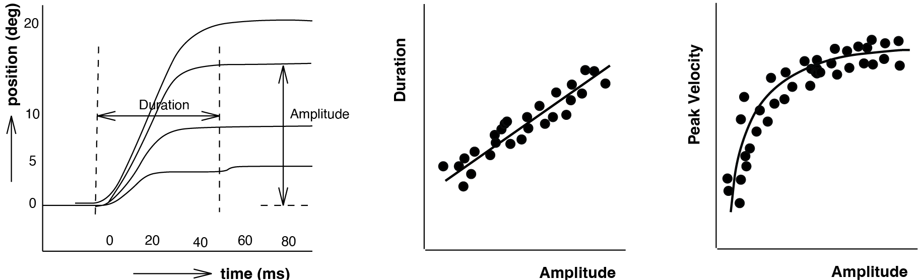
Fig. 56 | Saccade traces and main sequence

Typical position traces of saccades of different amplitudes. Larger saccades last longer, and their peak velocities saturate with amplitude—relationships collectively known as the saccadic main sequence.

The main sequence (Fig. 56) reveals that the saccadic system is fundamentally nonlinear: peak velocity does not scale proportionally with amplitude but instead saturates. In the previous module on the pulse–step generator (The Saccadic System - Pulse-Step Generator), we saw how the brainstem transforms a pulse-command into a signal that can drive the oculomotor plant. That signal consists of:

• a phasic pulse of high-frequency spikes → generates eye velocity,

• a tonic step of sustained activity → maintains eye position.

This pulse–step pattern is clearly visible in the firing of oculomotor motoneurons (Fig. 57):

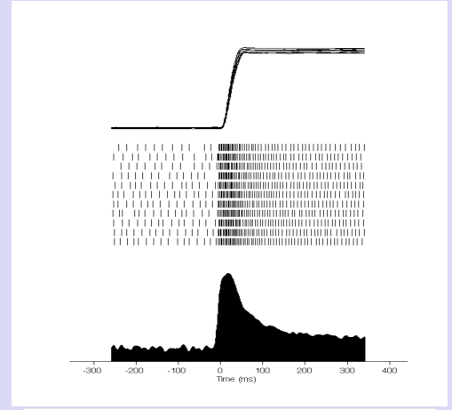
Fig. 57 | Pulse–step activity of oculomotor neurons.

A high-frequency phasic “pulse” drives a rapid eye movement, while the tonic “step” maintains the new eye position.

In the pulse–step module (The Saccadic System - Pulse-Step Generator), the focus was on how a pulse–step command can drive the oculomotor plant to produce fast and stable eye movements. The entire system considered there was fully linear: a phasic pulse entered a linear neural integrator (in NPH) to generate the tonic step, the pulse and step were combined through a linear summing pathway in the OMN, and the resulting command drove the oculomotor plant, which was modelled as a linear second-order low-pass filter (Fig. 58). Because each subsystem was linear, the overall input–output behaviour of the model was also linear. As a consequence, this architecture cannot explain the nonlinear properties of real saccades, such as the saturating peak velocities of the main sequence.

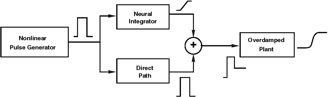
Fig. 58 | Pulse-step generator.

In this module, we expand the nonlinear pulse generator portion of the model (see Fig. 65). For the linear components, refer back to Fig. 44 and The Saccadic System - Pulse-Step Generator.

In the present module, we move one step upstream and focus on the Nonlinear Pulse Generator: where the pulse originates, how the brain computes it, and how its dynamics shape the saccadic eye movement.

What this module covers

The nonlinear pulse generator block in Fig. 58 consists of two key neural components (Fig. 59):

1. Long-Lead Burst Neurons (LLBNs) and

2. Short-Lead Excitatory and Inhibitory Burst Neurons (EBNs/IBNs).

Together, these structures generate the phasic pulse that drives the eye during a saccade. The LLBNs sit at the center of an internal feedback loop: they compare the desired eye displacement from the Superior Colliculus (SC) with an internal estimate of the ongoing eye movement. This produces the motor error, which is then transformed by the nonlinear EBN/IBN burst generator into an eye-velocity command (the pulse).

This system has two essential consequences:

1. Accuracy: saccades end precisely at the desired eye displacement specified by the SC due to the feedback loop inbvolving the LLBN,

2. Nonlinearity: the nonlinear EBN/IBN burst dynamics naturally reproduce the main-sequence relationships of real saccades.

These mechanisms — and the model that captures them — form the focus of this module.

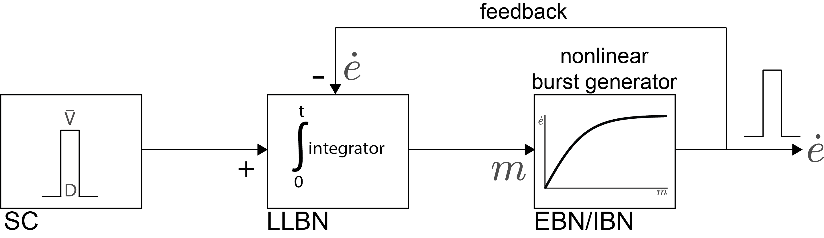
Fig. 59 | Simple scheme of the saccadic control system.

A simplified version of the 1-D Scudder model (1988). The Superior Colliculus (SC) specifies the desired eye displacement (\(\bar{V}\)). Long-Lead Burst Neurons (LLBNs) compare this desired displacement with an internal feedback estimate of ongoing eye velocity (\(\dot e \)). The resulting motor error (\(m\)) represents how far the eye still needs to move. Short-Lead Burst Neurons (EBNs/IBNs) convert this motor error into a nonlinear velocity command (\(\dot e\) vs \(m\)), generating the phasic pulse that drives the saccade.

Accuracy

Internal feedback in saccade generation

When a target appears on the peripheral retina, the saccadic system could, in principle, generate an eye movement based solely on the retinal error—the angular difference between the current gaze direction and the desired one. At first glance, this retinal error seems sufficient to guide an accurate saccade. However, classic work by Robinson and colleagues showed that visual feedback is far too slow to control saccades dynamically. Visual delays are on the order of 50–60 ms, which is comparable to or even longer than the duration of most saccades. Because saccades are both extremely rapid and remarkably accurate, their control must rely on mechanisms other than visual feedback alone. One early idea was that saccades might be generated by a fixed, preprogrammed motor pattern issued by the brainstem. While saccades indeed exhibit stereotyped kinematics, a large body of evidence demonstrates that the system also uses internal, non-visual feedback. This internal monitoring allows the brain to estimate the ongoing eye movement and adjust the motor command even when visual information is absent.

Multiple experimental observations support the existence of this internal feedback loop (see Fig. 60 and Fig. 61):

• Saccades remain accurate despite large trial-to-trial variability in their kinematics—for example due to drugs, fatigue, or perturbations (see Chapter Assignment: The Nonlinear Burst Generator, Fig. 76).
  If the system relied solely on a fixed preprogrammed burst, such variability would produce systematic dysmetria; instead, endpoints remain correct.

• Double-step paradigm in darkness:
  When two brief targets (A and B) are flashed and then extinguished, the system generates two accurate saccades (S1, S2) despite the absence of visual feedback. Remarkably, the second saccade is accurate even when target B is flashed during the first saccade (Fig. 60, top left). This requires the system to track the eye’s displacement during S1.

• Compensation for artificial eye displacement:
  If the eyes are moved during the reaction time by brief electrical microstimulation of the Superior Colliculus (SC), monkeys still produce an accurate saccade to the remembered target (Fig. 60, top right). Since the target is extinguished, the system must update its internal estimate of the starting eye position.

• Auditory-guided saccades in darkness:
  Accurate saccades can be made to sound sources even when no visual target is present. Because auditory space is encoded in head-centered coordinates, the saccadic system must know the eye’s absolute position in the orbit to translate head-centered target location into the appropriate eye-centered motor command.

• Interrupted saccades:
  Brief activation of the Omnipause Neurons (OPNs) can halt a saccade midflight (see Fig. 65). When OPN activity ceases, the saccade resumes and lands accurately on the invisible target (Fig. 60, bottom panel). This shows that the system retains an internal estimate of the remaining motor error, even when the movement is interrupted.

• Perturbation by blinks:
  Air-puff–induced blinks disrupt the kinematics of ongoing saccades, yet endpoints remain accurate (Fig. 61). This demonstrates that the system computes target location relative to an internally estimated eye trajectory rather than relying solely on the current visual input or a preprogrammed motor pattern.

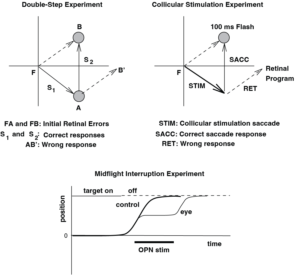
Fig. 60 | Evidence for internal feedback.

Top: Two experiments showing that internal (non-visual) feedback is used during saccade planning. Left: In the double-step paradigm, the second saccade is accurate even when the first saccade displaces the eyes unpredictably. Right: Electrical stimulation of the SC shifts the eyes during reaction time, but the resulting saccade still lands on the extinguished target. Bottom: Evidence for internal feedback during saccade execution. Brief activation of the OPNs stops the saccade midflight, yet when the burst resumes, the eye movement continues and reaches the correct target position. All experiments were performed in complete darkness, without visual feedback.

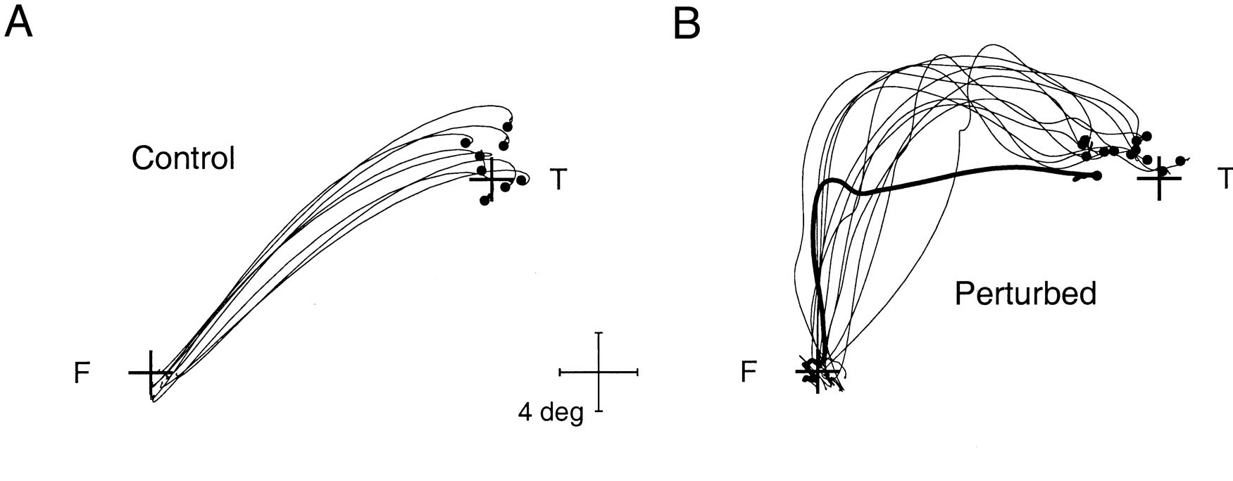
Fig. 61 | Blink-perturbed saccades.

A. Normal control saccades are accurate and go directly to target. B. An airpuff induces an eyelid blink, which perturbs the eye during the saccade. Still, the eye reaches its target in the end.

question – reference frame transformation

Why does the saccadic system need to know absolute eye position if it wants to make an eye movement to a sound source?

Solution

Auditory targets are encoded in a head-centered reference frame: the auditory system estimates the direction of a sound relative to the head, not relative to the fovea. To transform this head-centered sound direction into an appropriate eye-centered motor command, the brain must know where the eyes currently are in the orbit.

If the eyes are already deviated left or right when the sound occurs, the required saccade amplitude and direction change accordingly. Without knowledge of absolute eye position, the system could not correctly convert:

\(\text{sound direction (head-centered)} \quad \longrightarrow \quad \text{desired change in gaze (eye-centered)}\).

Thus, accurate auditory-guided saccades require an internal estimate of the current eye position to compute the correct motor error and resulting saccade vector.

Feedback

Two concepts are essential for understanding the burst generator: internal feedback and velocity integration. In this section we develop an intuition for why internal feedback is needed, using a simple mathematical example before returning to the saccadic system.

Feedback is ubiquitous in biological systems. Its prevalence is not accidental. Feedback increases

• robustness (the system keeps working even when components vary),

• accuracy (errors are continuously corrected), and

• insensitivity to noise or parameter drift (e.g. muscle fatigue, neural variability).

To illustrate these properties, consider the simple negative-feedback loop shown in Fig. 62. The system contains a forward gain \(G\) and a feedback gain \(H\), both linear and positive. The input \(X(t)\) is compared to a scaled version of the output \(Y(t)\), and the resulting error signal is passed through the forward pathway.

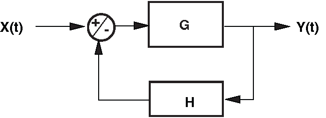
Fig. 62 Simple negative-feedback system with forward gain \(G\) and feedback gain \(H\).

Mathematically, the overall input–output relation is:

\[\frac{Y}{X} = \frac{G}{1 + G \cdot H}.\]

question – gain of simple feedback system

Show that the transfer characteristic (relation between input \(X\) and output \(Y\); closed-loop gain) of the system is:

\[\frac{Y}{X} = \frac{G}{1 + G \cdot H}.\]

Solution

We derive the closed-loop gain by writing down the signals at each node and then eliminating the intermediate variables.

1. Label the intermediate signals

Let

• \(U\) = signal after the summing junction (error signal),

• \(V\) = feedback signal after the block with gain \(H\).

The other signals are the input \(X\) and the output \(Y\).

2. Write down the relations between signals

From the diagram in Fig. 62:

• Summing junction (negative feedback):
  \( U = X - V \)

• Forward path with gain \(G\):
  \( Y = G \cdot U \)

• Feedback path with gain \(H\):
  \( V = H \cdot Y \)

3. Substitute and simplify

First substitute \(V = H Y\) into the expression for \(U\): \( U = X - H Y. \)

Now substitute this \(U\) into the expression for \(Y\): \( Y = G \cdot U = G \bigl(X - H Y\bigr). \)

Expand the right-hand side: \( Y = G X - G H Y. \)

Collect the terms in \(Y\) on the left-hand side: \( Y + G H Y = G X, \) \( (1 + G H)\,Y = G X. \)

Finally, divide both sides by \(X\) and by \((1 + G H)\): \( \frac{Y}{X} = \frac{G}{1 + G H}. \)

Thus, the closed-loop gain of the negative-feedback system is: \( \boxed{\dfrac{Y}{X} = \dfrac{G}{1 + G H}}. \)

why this matters biologically

If \(G\) is large then the product \(G \cdot H\) is large. The denominator then becomes: \(GH\) instead of \(1+GH\).

The full equation then becomes

\[\frac{Y}{X} \approx \frac{1}{H}\]

which is independent of the forward gain \(G\) and depends almost exclusively on the feedback gain \(H\).

First, consider the case that \(H = 1\). If \(G\) is large enough, the closed-loop gain approaches 1, meaning the system reproduces the input accurately regardless of variations in \(G\).

Now consider the case where H represents an upstream subsystem, such as the oculomotor plant or any downstream stage whose properties might vary. In the large-gain limit, the closed-loop gain \(\frac{1}{H}\) effectively cancels out the influence of that subsystem, \(\frac{1}{H} \cdot H = 1\). In other words, the negative-feedback loop forces the overall behaviour to follow the reference input, regardless of variability or imperfections in the downstream machinery.

This has powerful implications for biological motor systems:

• Even if the forward pathway weakens (due to fatigue, neuromodulation, or drug effects),

• and even if individual components fluctuate from trial to trial,

the overall sensorimotor transformation remains stable and accurate.

The same principle applies directly to the saccadic system:

• Burst neuron firing rates vary from trial to trial,

• muscle contractile strength changes with fatigue,

• and neural activity is inherently noisy.

Yet saccades land accurately and consistently. This is because the LLBN–EBN/IBN circuit forms a negative-feedback loop, continuously computing motor error and adjusting the drive to the motoneurons until the error becomes zero. In other words, the system does not rely on a brittle, preprogrammed burst — it actively corrects itself.

question - positive feedback

What happens if the feedback is positive rather than negative? (Hint: Think about stability.)

solution - Why positive feedback is unstable

With positive feedback, the summing junction becomes

\(U = X + HY\),

and the closed-loop gain becomes

\(\frac{Y}{X} = \frac{G}{1 - GH}.\)

1. Behaviour when \(G \gg 1\)

If the forward gain is very large, then \(GH\) is also large. The denominator is dominated by \(-GH\), giving:

\(\frac{Y}{X} \approx -\frac{1}{H}\).

This gain is

• independent of \(G\) (just as in negative feedback),

• but negative, meaning the signal is inverted,

• and importantly, it does not suppress deviations—it amplifies them.

2. Special case: \(H = 1\) and \(G \gg 1\)

Then \( \frac{Y}{X} \approx -1. \)

The system feeds back the output with equal magnitude but opposite sign, and then adds it to the input.
This does not cancel errors — it causes them to grow. Even tiny noise produces oscillations or runaway outputs.

3. Instability when \(GH \to 1\)

As the product \(GH\) approaches 1:

\(1 - GH \to 0 \quad\Rightarrow\quad \frac{Y}{X} \to \infty,\)

so the system becomes extremely sensitive: even microscopic disturbances get amplified enormously.

4. Summary: positive feedback destabilizes

• Small deviations are reinforced, not corrected.

• Noise and parameter variability are amplified.

• For \(GH > 1\), outputs can diverge or oscillate without bound.

5. Biological relevance

Such behaviour would be disastrous for the saccadic system:
errors in eye-position estimation or burst firing would grow rather than be corrected, and the eyes would fail to land stably on the target. This is why the LLBN–EBN/IBN circuit uses negative, not positive, feedback.

Long-Lead Burst Neurons (LLBNs) – computing motor error

The negative-feedback principle discussed above is implemented biologically in the Long-Lead Burst Neurons (LLBNs) (see Fig. 63). The LLBNs compare two key signals:

• a desired drive from the Superior Colliculus (SC), and

• an internal feedback signal proportional to the ongoing eye velocity \(\dot e(t)\), supplied by the short-lead burst neurons (EBNs).

The LLBNs compute the difference between these two signals and integrate it over time:

(23)\[m(t) = \int_0^t \big[\,SC(\tau) - \dot e(\tau)\,\big]\,d\tau\]

This integration has a clear interpretation. If we assume that the motor error returns to zero at the end of the movement, we can rewrite the equation as:

(24)\[m(t) = \Delta e_d - \Delta e(t),\]

where

• \(\Delta e_d = \int_0^t SC(\tau)d\tau\) is the desired eye displacement (encoded by the total spike count of the SC burst), and

• \(\Delta e(t) = \int_0^t \dot e(\tau)d\tau\) is the actual displacement executed so far.

Thus, both expressions describe the same quantity:

• Equation (23) expresses motor error as the dynamic integral of desired velocity minus actual velocity,

• whereas equation (24) expresses it geometrically as the difference between desired and achieved displacement.

In essence, the LLBNs integrate how much of the desired movement remains at each moment. Their output, \(m(t)\), is the instantaneous motor error. When \(m(t)\) reaches zero, no further movement is required — the saccade ends.

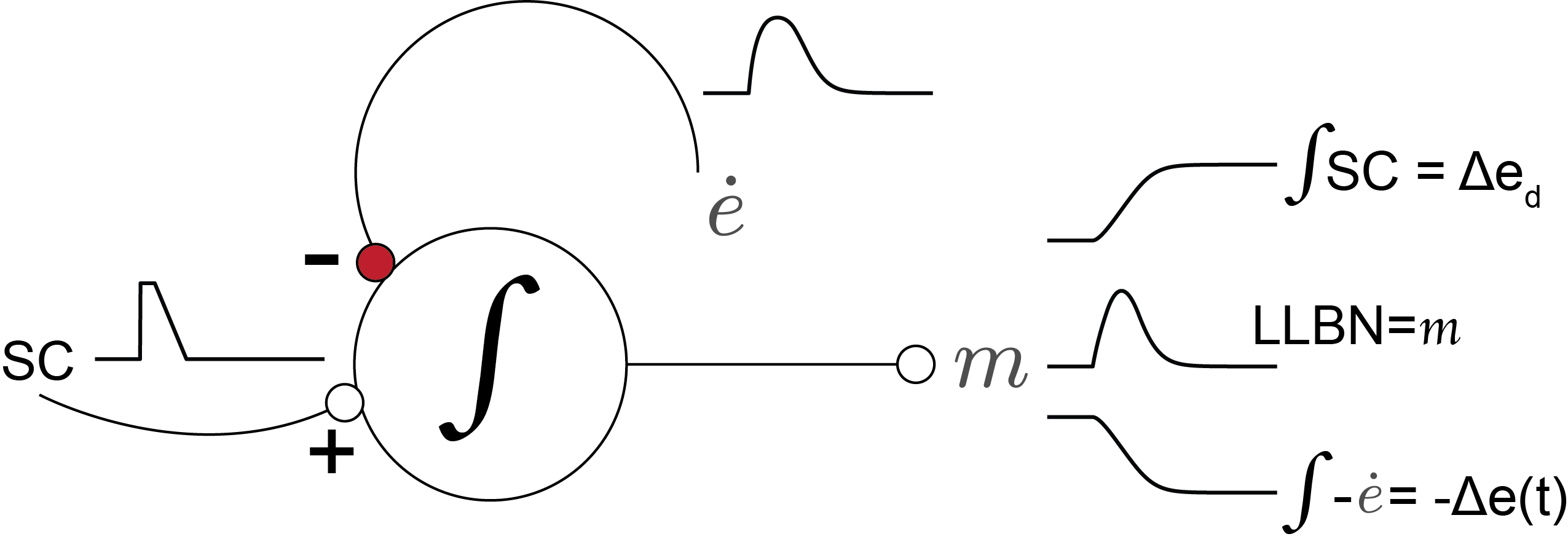
Fig. 63 | Long-Lead Burst Neurons (LLBNs).

The LLBNs implement the system’s internal feedback loop. They compare the desired drive from the SC with an internal estimate of ongoing eye velocity from the burst neurons (EBNs), and integrate the difference. Because the spike count of the SC burst encodes desired eye displacement \(\Delta e_d\), the LLBN output \(m(t)\) corresponds to the remaining motor error: the difference between desired and achieved displacement. Their output drives the short-lead burst neurons (EBNs/IBNs), which generate the phasic saccadic pulse.

Download Matlab code to simulate LLBN feedback

Non-linearity

Short-Lead Burst Neurons (EBNs & IBNs) generating the pulse

Up to this point, all elements of the saccadic system have been linear:

• the LLBN integrator is linear (integration is a linear operation),

• the internal feedback loop is linear,

• and the downstream pathways that summate and hold the signal are also linear.

This raises an important question:

Where do the nonlinear properties of saccades come from?

A major source of nonlinearity is the short-lead burst neurons—the Excitatory and Inhibitory Burst Neurons (EBNs and IBNs). These neurons exhibit a saturating input–output characteristic (Fig. 64): their firing rate cannot increase indefinitely but approaches an asymptote.The relationship between motor error \(m(t)\) from the LLBNs and the eye-velocity (pulse) command \(\dot e(t)\) produced by the burst generator is:

(25)\[\dot e(t) = E_0 \left[ 1 - e^{-\,m(t)/e_0} \right],\]

where

• \(E_0\) is the maximum attainable eye velocity (the asymptote), and

• \(e_0\) sets the slope of the nonlinearity (how quickly saturation is approached).

For small values of \(m(t)\), the exponential term is nearly linear, and:

\(\dot e(t) \approx \frac{E_0}{e_0} \cdot m(t)\)

But as motor error \(m(t)\) increases, the exponential term flattens out, and eye velocity \(\dot e(t)\) grows more slowly, eventually approaching the asymptotic velocity \(E_0\).

Fig. 64 | Short-Lead Burst Neurons.

A. Nonlinear input–output characteristic of the short-lead burst neurons (EBNs/IBNs). The burst generator transforms motor error \(m\) into eye velocity \(\dot e\) through a saturating exponential (Eq. (25)). For small motor errors the mapping is approximately linear, but as \(m\) increases the output approaches a maximum velocity \(\dot e_{max}\). The parameter \(m_0\) indicates the motor-error level at which the output reaches 63% of its maximum value \((1 - e^{-1} = 0.6321)\).

B. Time course of the motor error \(m(t)\) generated by the LLBNs. Open circles with numbers mark consecutive moments during the saccade, illustrating how the motor error evolves over time as the desired displacement is gradually reduced.

C. The same numbered moments plotted on the burst-generator nonlinearity. Early in the movement (large \(m\), 1-3), the system operates in the saturated region where increases in motor error produce little change in eye velocity. Later, as \(m\) decreases (4-6), the operating point moves back into the more linear portion of the curve. Compare these operating points directly with the time course shown in panel B.

Download Matlab code to generate components of this figure

question – why is this nonlinear?

Why is the mapping from \(m(t)\) to \(\dot e(t)\) considered nonlinear?

Solution

Because the mapping does not obey the superposition principle. If you multiply the input \(m(t)\) by a factor \(a\), the output \(\dot e(t)\) does not scale by the same factor.

For example:

\[\dot e(t) = E_0\big(1 - e^{-m/e_0}\big), \qquad \dot e_a(t) = E_0\big(1 - e^{-a \cdot m/e_0}\big).\]

For large \(m\), both approach the same asymptote \(E_0\), regardless of the scaling factor \(a\). A linear system would produce \(a \cdot \dot e(t)\), which clearly does not occur here.

How LLBN output and burst saturation interact

The output of the LLBNs is the motor error, which evolves dynamically:

• At saccade onset, \(m(t)\) is small (process has not started yet).

• Then \(m(t)\) grows rapidly (desired displacement > actual displacement).

• As the eye moves, \(m(t)\) gradually decreases back toward zero.

The nonlinear mapping of the burst neurons affects these phases differently:

• At movement onset: For small motor errors, the relation is almost linear → eye velocity increases steeply and closely follows \(m(t)\).

• During mid-flight: As \(m(t)\) becomes larger, the burst generator saturates → even large increases in \(m(t)\) produce only modest increases in \(\dot e(t)\) (Fig. 64C, moment 1→3).

• Near the end of the saccade: As \(m(t)\) becomes small again, the system becomes linear again → \(\dot e(t)\) closely reflects the remaining motor error until it reaches zero (Fig. 64C, moment 4→6).

This interaction shapes the saccadic main sequence:

• Larger desired displacements produce larger motor errors, → but due to saturation, eye velocity approaches a maximum.

Therefore:

• peak velocity increases with amplitude (but not proportionally),

• peak velocity saturates for large saccades,

• duration must increase for larger saccades (because velocity cannot increase further).

In short, the saturating nonlinearity of EBNs/IBNs provides a simple and elegant explanation for the characteristic nonlinear relations observed in saccades.

A Quantitative Model of the Saccadic System

The Full Model

We can now assemble the pieces introduced so far. The Long-Lead Burst Neurons compute the instantaneous motor error (see Fig. 63), the short-lead burst neurons (EBNs/IBNs) convert this motor error into a nonlinear pulse (see Fig. 64), and the pulse–step pathway from the previous module (Fig. 58, The Saccadic System - Pulse-Step Generator) transforms this pulse into the motoneuron activity that drives the oculomotor plant.

Together, these components form the classical 1-D saccade model proposed by Scudder (1988) (Fig. 59). Integrating the burst-generator block with the final common pathway yields the complete model (Fig. 65), capable of producing saccades that are fast, accurate, and that naturally reproduce the main-sequence nonlinearities. The expanded model (Fig. 65) includes the following functional elements:

• Desired eye displacement from the Superior Colliculus (SC)

• Motor error, computed by the LLBNs, as the integrated difference between desired drive and internal feedback

• Pulse generation by the nonlinear EBNs/IBNs

• Neural integration producing the tonic step

• Summation of pulse and step in the oculomotor neurons (OMNs)

• The oculomotor plant, producing the actual eye movement

• Gating by the Omnipause Neurons (OPNs), ensuring proper saccade onset and termination

These interacting subsystems together form a compact but powerful description of saccadic control.

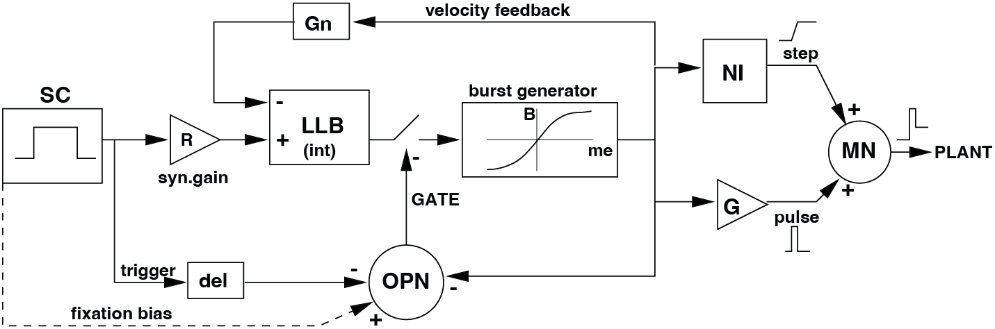
Fig. 65 | Saccade control model.

The complete 1-D saccadic system. The Superior Colliculus (SC) specifies the desired eye displacement. LLBNs compute the motor error by comparing SC drive with an internal feedback estimate. Short-lead burst neurons (EBNs/IBNs) transform the motor error into a nonlinear pulse. OPNs gate the system by inhibiting burst neurons during fixation. Pulse and step are combined in the motoneurons to drive the oculomotor plant.

Omnipause Neurons (OPNs) – the saccadic gate

One element not yet discussed in detail in this module (see The Saccadic System - Pulse-Step Generator) is the Omnipause Neurons. OPNs provide a powerful gating mechanism:

• During fixation: OPNs fire continuously and inhibit all burst neurons, preventing accidental saccades.

• At saccade onset: OPNs pause, releasing the EBNs and IBNs to generate the high-frequency pulse.

• At saccade end: OPNs resume firing, shutting down the burst generator and ensuring a sharp, ballistic termination.

Without OPNs, the burst generator would not be reliably switched on and off, and saccades would not be discrete, well-timed movements.

question – OPN gating

Why is the gating action of the Omnipause Neurons (OPNs) considered nonlinear?

Solution

Because OPNs implement a threshold-based, all-or-none switch, which does not obey the superposition principle.

• When OPNs fire, they completely suppress activity in the burst neurons (EBNs/IBNs).

• When their firing pauses, the inhibition is fully released, allowing the burst generator to activate.

This is a binary gating operation:
either inhibited or disinhibited, with no intermediate graded response.

If the input to the OPNs is scaled (e.g., doubled), the output does not scale proportionally—
the gate is still either closed (burst neurons fully inhibited) or open (burst neurons fully active), depending only on whether the threshold is crossed.

Such threshold-based switching is inherently nonlinear, because it violates superposition and cannot be expressed as a linear transformation of the input.

The Superior Colliculus

The Superior Colliculus (SC) provides the desired eye-displacement command that initiates the saccadic cascade. The SC contains a two-dimensional map of saccade vectors (which is covered in detail in The Saccadic System - Superior Colliculus). The site and extent of neural activation in this map determine:

• the direction of the desired eye movement,

• the amplitude of the movement (encoded by the number of spikes in the burst), and

• the speed profile of the drive (related to the burst’s temporal shape).

This desired vector is then transformed by the brainstem circuit into the actual motor command that moves the eyes.

Follow-up

In the computer practical (Assignment: The Nonlinear Burst Generator), you will implement and experiment with this full saccade model — combining the LLBN feedback loop, the burst-generator nonlinearity, the pulse–step pathway, and the oculomotor plant. You will explore how each component affects the accuracy, speed, and dynamics of the resulting saccades.

In the next module (The Saccadic System - Superior Colliculus), we turn upstream and examine how the Superior Colliculus encodes desired eye movements, and how its spatial map organizes saccades.

Background: The Common Source for 2D saccades

Two-dimensional eye movements: the Common Source Model

Up to now we have considered a one-dimensional model of the saccadic system. In reality, eye movements are two-dimensional (horizontal + vertical), and even include a small torsional component For simplicity, we ignore torsion here and focus only on horizontal–vertical movements.

The challenge of controlling 2-D saccades

Vertical saccades are generated by burst neurons in the medial longitudinal fasciculus (MLF) and held by a neural integrator in the interstitial nucleus of Cajal (INC), whereas horizontal saccades rely on the PPRF and the NPH/MVN integrator. Neurophysiology shows that these two systems operate in parallel and are tuned to orthogonal movement directions. Yet, when we make an oblique saccade, the eye does not move as if two independent 1-D controllers were simply added together. Instead:

• horizontal and vertical components begin and end at almost the same time,

• the resulting saccade trajectory is approximately straight,

• and the peak velocities of the components obey the same main-sequence constraints.

This requires a shared command upstream of the horizontal and vertical pulse–step generators.

The Superior Colliculus as the common input

Both horizontal and vertical burst generators receive a common signal from the Superior Colliculus (SC). The SC encodes a vectorial desired eye displacement \(\Delta \mathbf{e}_d\) in a topographic motor map: the location of activity on the map specifies the direction and amplitude of the intended saccade. This vectorial command must be transformed into two separate neural commands for the horizontal and vertical eye muscles. This transformation is known as the spatial–temporal transformation.

Spatial–temporal transformation

This process can be separated into two conceptual stages:

1. Spatial (vector) transformation – converting the desired displacement vector
   \((\Delta e_d \cdot \Phi)\) into its horizontal and vertical components: \(\Delta H = R \cos\Phi, \qquad \Delta V = R \sin\Phi\).

2. Temporal transformation – converting the time-varying motor error \(m(t)\) into the required eye-velocity command \(\dot e(t)\) using the nonlinear burst generator.

The first step, vector decomposition (VD), is linear.
The second step, pulse generation (PG), is nonlinear, e.g.

\(\dot e = a\left(1 - e^{-b m}\right),\)

which produces the main-sequence kinematics.

Because one process is linear and the other is nonlinear, the order matters:

\(VD \circ PG \neq PG \circ VD .\)

Evidence from oblique saccades

Studies of oblique saccades show:

• horizontal and vertical velocity profiles are tightly matched in duration,

• the resulting eye movement is nearly straight,

• and both components exhibit the same nonlinear saturation.

A simple way to achieve this is to assume that the pulse generator produces a vectorial eye-velocity signal, which is then decomposed into horizontal and vertical components. This is the essence of the Common Source Model:

A single vectorial burst generator (the PG stage) produces a velocity vector whose direction and length encode the desired 2-D eye-velocity profile; this vector is subsequently decomposed (VD stage) into horizontal and vertical components to drive the respective burst generators.

Under this scheme:

• both components share the same motor error time course,

• both end when the motor error reaches zero,

• and trajectories remain approximately straight.

Relevant structures in the brain

To orient yourself to the anatomical context of these transformations, the figures below show simplified schematics of gaze-control areas in the monkey (and human) brain.

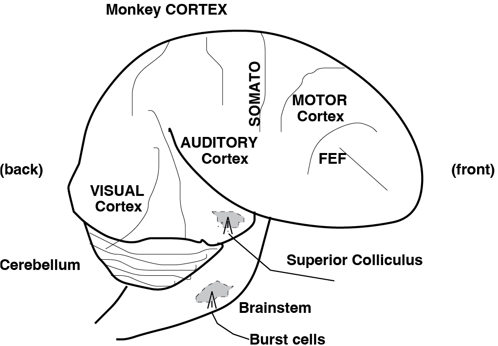
Fig. 66 | Gaze control in the CNS

Side view of the monkey brain with key gaze-control regions: visual cortex, auditory cortex, motor cortex, cerebellum, and brainstem. FEF: frontal eye fields; Somato: somatosensory cortex. The human brain has a very similar organization.

The next figure places these structures in the full visual → sensorimotor → motor pathway.

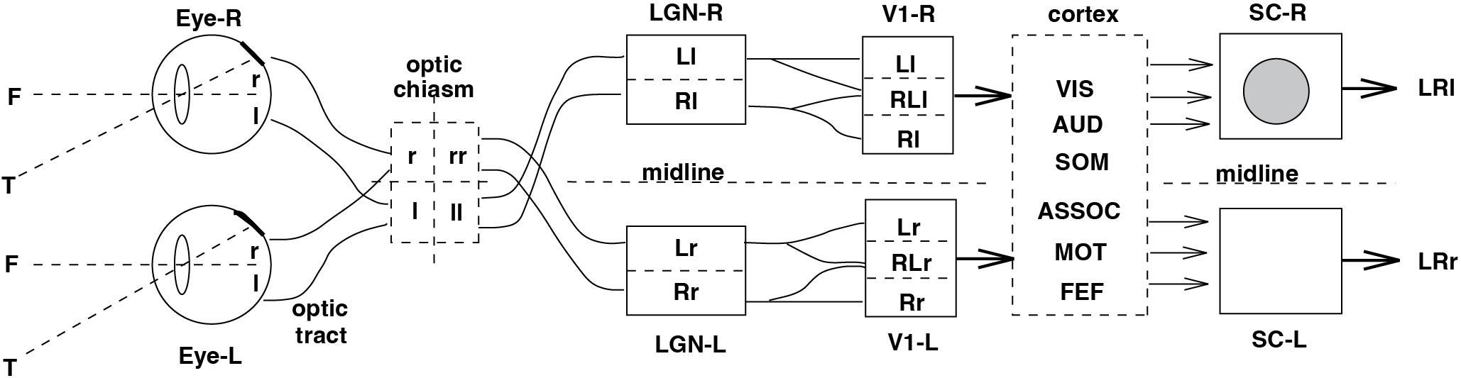
Fig. 67 :name: fig_neuralscheme_saccade | Neural structures leading to goal-directed eye movements

Schematic overview of the cortical, subcortical, and brainstem structures involved in generating a goal-directed saccade. Visual signals from the retina are processed in the retina, chiasm, LGN, and V1, and ultimately converge on sensorimotor structures including parietal cortex, FEF, and the SC. The SC then drives the brainstem saccade generator.

Summary

For two-dimensional saccades, the brain does not run two independent 1-D controllers. Instead:

• a vectorial desired movement is encoded in the SC,

• a common, nonlinear pulse generator produces a 2-D velocity vector,

• and only then is the vector decomposed into horizontal and vertical muscle commands.

This Common Source architecture naturally explains the tight synchrony, straight trajectories, and unified main-sequence kinematics of oblique saccades.

question – Common Source

In the ‘Common Source’ model of the saccadic system (e.g. Fig. 59 and Fig. 65), the brainstem is driven by a nonlinear vectorial pulse generator that transforms a 2D motor error vector, \(\Delta e_{vec}\), into a vectorial eye-velocity command according to: \(\dot e_{vec}(t) = v_{max} \cdot [1 - \exp{-\frac{\lvert \Delta e_{vec}(t) \rvert }{m_o}}]\) with \(\lvert \cdot \rvert\) the magnitude of the vector. Give expressions for the velocity profiles of oblique saccades \([R,\phi]\), with identical horizontal saccade components (i.e. horizontal component amplitude is fixed, say at \(\Delta H\), but the vector rotates over angle \(\phi\) with respect to the horizontal direction).