Assignment: The Linear Pulse-Step generator#
Learning Goals#
Learning goals
In this computer practical you will explore how a saccadic system transforms a neural pulse–step command into a fast and accurate eye movement. Using the simplified Pulse–Step Generator Simulink model (pulsestep.slx), you will:
Apply core concepts from systems theory:
linearity and superposition
feedforward vs feedback pathways
the role of system time constants
Understand the distinct functional roles of:
Burst neurons (EBN/IBN) – generating the pulse
Neural integrator – generating the step
Direct (feedforward) pathway
Oculomotor plant – the biomechanics of the eye
Inverse model – reconstructing motor commands
Predict and interpret the effects of simulated brainstem “lesions”:
Integrator failure
Plant parameter changes
Pulse–step mismatch
By interactively changing model parameters and analysing the output, you will develop intuition for the dynamics underlying saccadic eye movements.
Data#
Downloads#
Download the Matlab files:
This contains the Pulse-Step model, which is a model of the final stage of the saccadic system as discussed in The Saccadic System - Pulse-Step Generator.
Research Data Management#
To keep your work organised and reproducible, set up a simple folder structure before you begin:
Create a main folder named NBP_pulsestep.
Inside this folder, create three subfolders:
data – for storing exported simulation data files
analysis – for your MATLAB scripts and the Simulink model
figures – for saving plots and exported images
Place the Simulink model and all MATLAB code in the analysis folder. Then create a new MATLAB script named data_analysis.m in this folder. You will use this script to run your simulations, analyse the output, and generate figures. Whenever your script produces data files or images, save them into the corresponding data or figures folder. This structure helps ensure your work is easy to navigate, reproducible, and ready for future assignments. For additional guidance, see Research Data Management.
Working With Simulink#
This practical uses Simulink. Simulink is MATLAB’s graphical environment for building and simulating dynamic systems. Instead of writing equations in code, you create models by connecting functional blocks that represent mathematical operations, neural circuits, or physical systems. Many biological systems—including the saccadic pulse–step generator—can be described as continuous-time, dynamic systems with:
inputs (e.g., neural pulse signals)
internal computations (e.g., integration, time constants)
outputs (e.g., eye position and velocity)
Simulink lets you:
visualize the components (neurons, integrators, plant dynamics)
modify parameters interactively
see the consequences immediately in scopes
simulate continuous time without manually coding differential equations
This makes it ideal for understanding how the brain generates precise movements.
Opening the Model#
Start MATLAB.
In the Command Window, type (or put this in a script and run that script):
open_system("pulsestep.slx")
The top-level Simulink diagram will open.
Running Simulations#
Click Run ( ▶ ) in the Simulink toolbar.
The default simulation time is 0.5 s, which is appropriate for saccades.
Viewing Signals#
After clicking Run, Scopes will appear that contain the signals generated by the simulation.
Editing Parameters#
Double-click any subsystem block:
Burst Generator
Neural Integrator
Direct Path
Oculomotor Plant
Inverse Plant Model
Then edit the parameters (e.g., P, D, Gain, T1, T2).
Use correct units: seconds, milliseconds, spikes/s, dimensionless gains.
Creating a Figure#
To create a figure of a Scope in a Word-document, you can right-click on the scope and choose “Print Display to Figure”, which creates a Matlab Figure. You can copy that figure (click on Figure>Copy Figure) and paste this into the Word-document.
MATLAB#
In this tutorial, you will receive MATLAB code that automates the simulations required for each assignment. However, make sure to actively explore the Simulink model yourself:
double-click blocks to inspect and change parameters,
view and measure the signals in the Scopes or Data Inspector,
and reason about how each subsystem affects the final eye-movement output.
The goal is not only to run the scripts, but to understand how this model represents the final stages of the saccadic system, and how changes in pulse, step, and plant dynamics shape the behavior of real saccades.
Computer exercises with the linear PulseStep generator model#
These exercises introduce you to the behaviour of the pulse–step generator and the principles of linear system analysis. We will inspect a simple model of the so-called ‘Final Common Pathway’ of the oculomotor system (Fig. 50) is also available under Simulink as file pulsestep.slx (Fig. 51 and Fig. 52). This simulation model, allows you to interactively set parameters of:
The saccadic burst from the EBNs/IBNs (this is simply modeled as a pulse, having a height, \(P\), and duration \(D\).)
The neural integrator: setting its gain to zero mimics total loss of the integrator, whereas a gain of one means normal operation.
The direct path: feeds the pulse directly to the oculomotor neurons. When its gain is set to zero, you actually simulate the effect of a Step input to the OMNs.
The Plant, with its two time constants, \(T_1\) and \(T_2\)
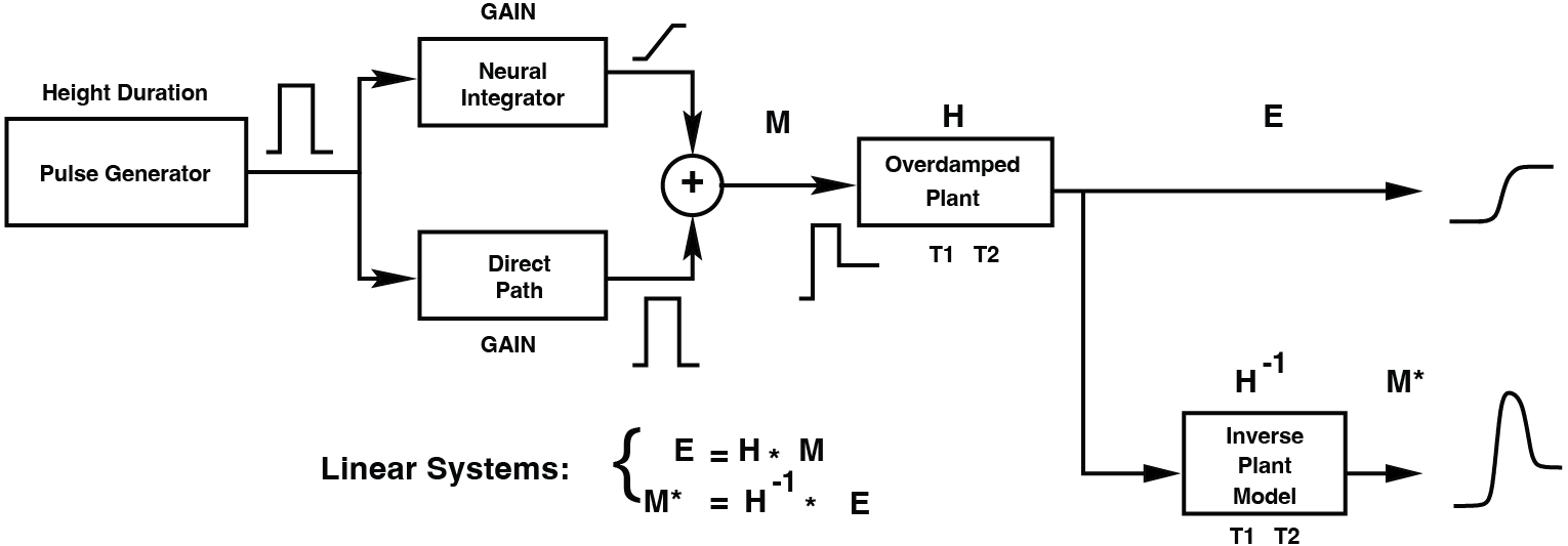
Fig. 50 | Model for the Final Pathway of the Oculomotor System#
For saccades, this embodies the Pulse-Step Generator. The output of this pathway (i.e. eye position) is subsequently fed through an Inverse Model of the Plant, to enable a reconstruction of the motoneuron signal (see also Fig. 75)
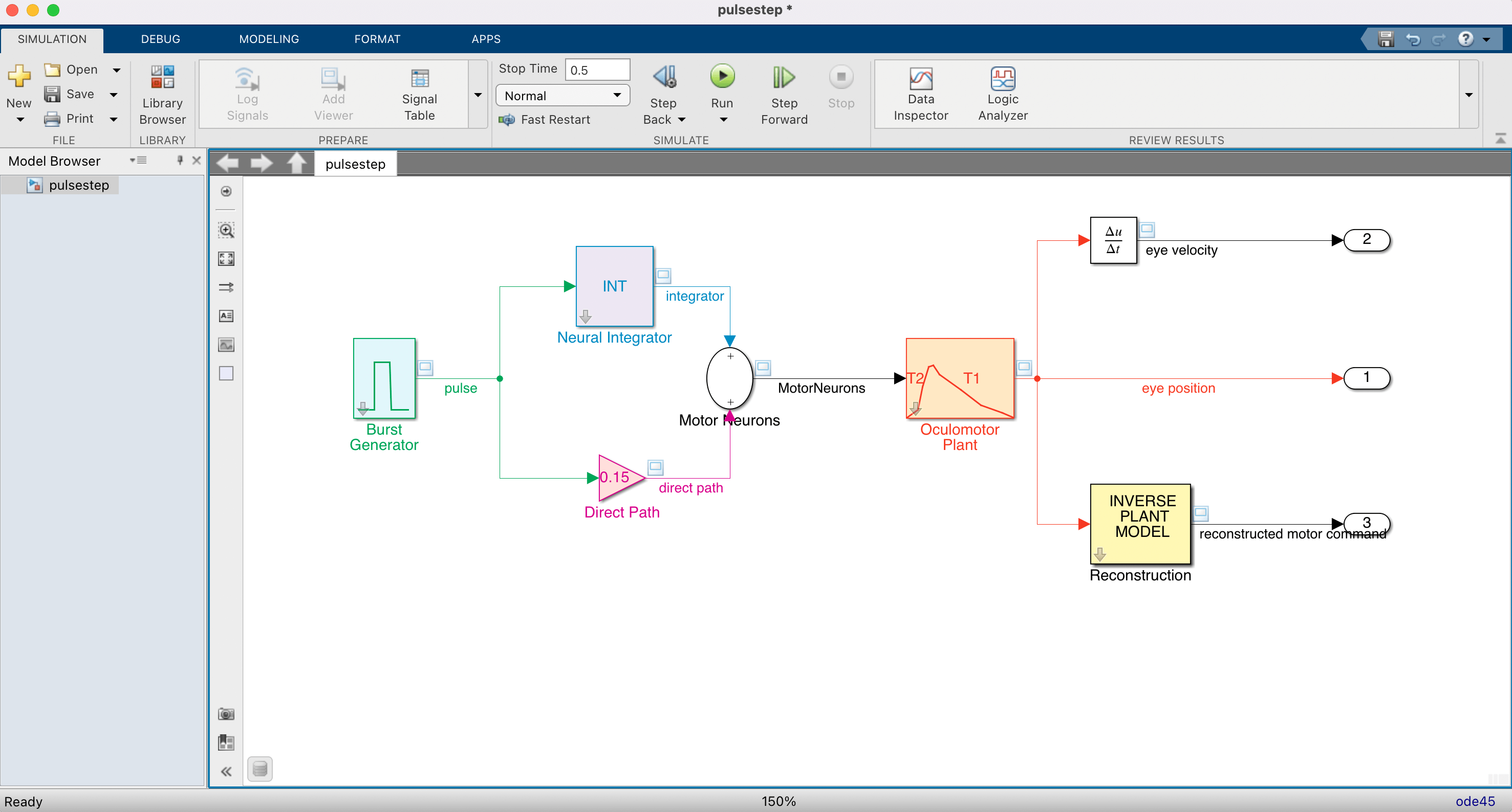
Fig. 51 | PulseStep Simulink Model.#
Compare to Fig. Fig. 50
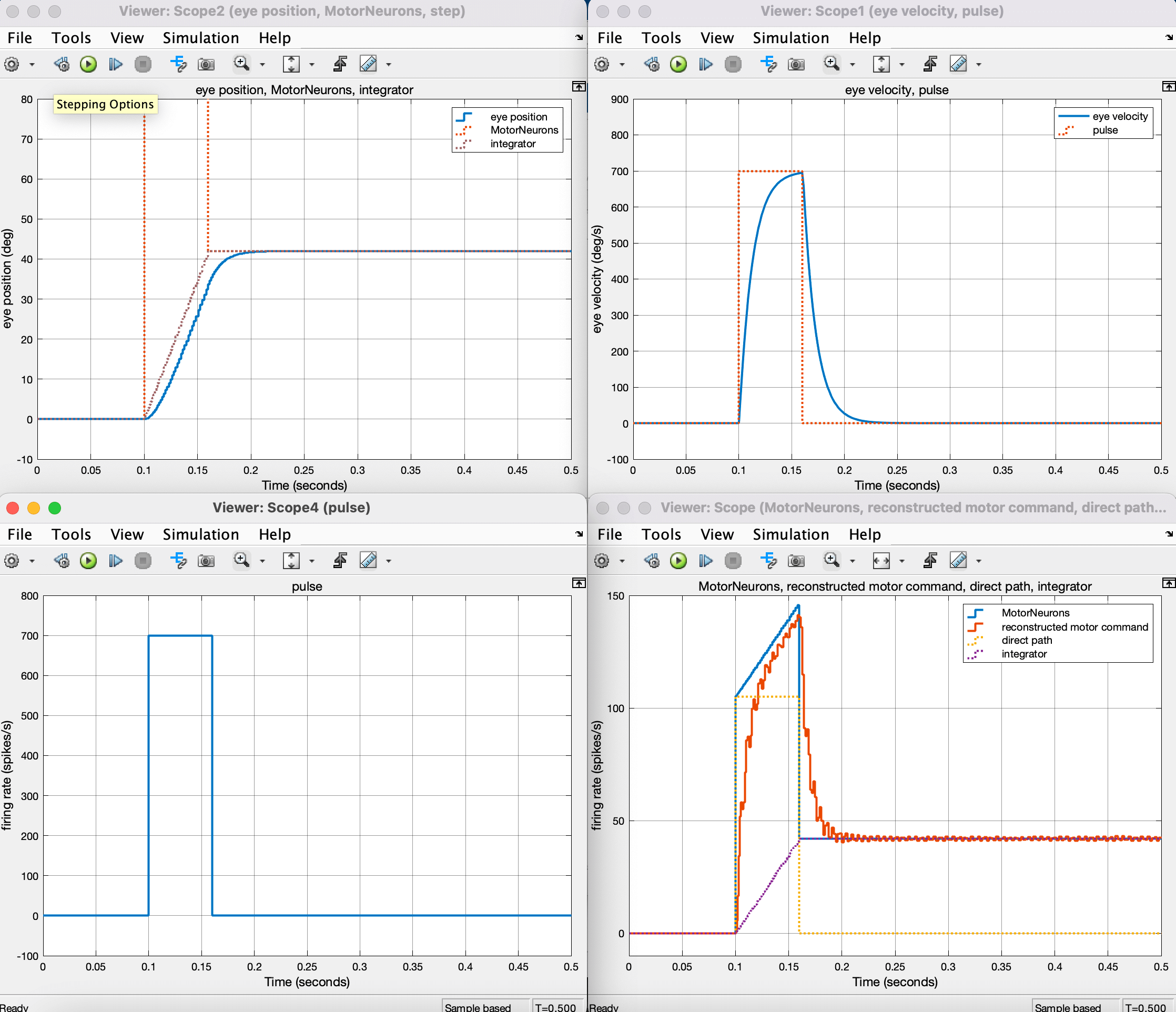
Fig. 52 Scopes in the PulseStep Model.#
Exercise 1 — Saccade Amplitude#
Run the model.
%% Pulse–Step Generator – MATLAB/Simulink Helper Script
% This script loads the Simulink model 'pulsestep.slx', sets parameters,
% runs simulations, and extracts the logged signals EyePos, EyeVel, Command.

clear; close all; clc;

modelName = "pulsestep";

%% 1. Load and open the model
load_system(modelName);
open_system(modelName);


%% 2. Set default parameter values
psg_set_default_params(modelName);

%% PRESS RUN
One of the scopes should look like Fig. 53. To get some measurement guides, you need to go to MEASUREMENTS (Fig. 54), and click on Data Cursors. You can now click and drag the measurement guides and inspect relevant values (Fig. 55).
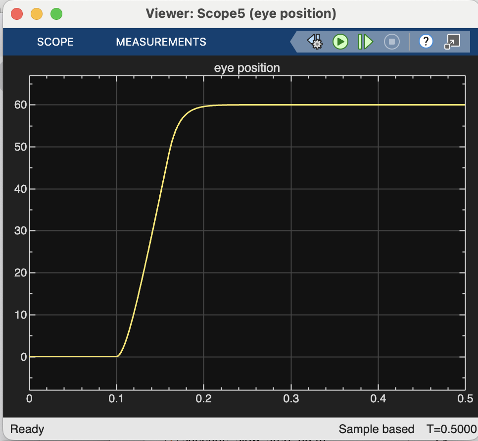
Fig. 53 | Eye Position Trace#
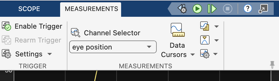
Fig. 54 | Measurement toolbar#
Click on Data Cursors.
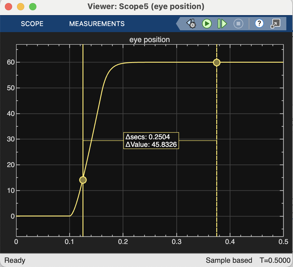
Fig. 55 | Measurement tools#
Move the guides to points of interest.
Determine the amplitude of a saccade from the eye-position trace using the guides (Look at the difference between the final and initial position.)
How does this relate to the underlying pulse–step command?
MATLAB Code
%% Exercise 1: Saccade Amplitude
Amplitude = EyePos(end) - EyePos(1);
disp(Amplitude)
Exercise 2 — Exploring Model Parameters#
Interactively change the following parameters, one at a time, while keeping all others at their default values:
Burst Generator:
Pulse height \(P\) (spikes/s)
Pulse duration \(D\) (s)
Neural Integrator:
Integrator gain
Direct Pathway:
Forward gain
Oculomotor Plant:
Long time constant \(T_1\)
Short time constant \(T_2\)
You can set the default parameters by:
%% 2. Set default parameter values
psg_set_default_params(modelName);
For each parameter change, note:
How large is the saccade amplitude?
What is the peak velocity?
What is the saccade duration?
How does the pulse–step output change?
Does the eye movement remain accurate?
Accuracy refers to whether the eye reaches and maintains the intended final position of the saccade.
If the goal is 20°, then a saccade is accurate when its final eye position is 20°.
In the Pulse–Step model, the burst parameters (pulse height P and pulse duration D) determine the desired amplitude of the saccade. Changing P or D therefore changes the goal and will naturally lead to a different final amplitude.
To study accuracy, you should therefore: 1. Set a target amplitude using P and D (e.g., make a 20° saccade). 2. Keep P and D fixed, and then vary the other parameters:
Then observe:
Does the saccade still end at the intended position?
Is there an overshoot or undershoot?
Does the eye drift back toward centre after reaching the target?
Does the final position depend systematically on the parameter you changed?
Exercise 3 — Linearity#
A system is linear if for all inputs \(x(t)\), \(y(t)\) and constants \(a,b\):
Simulate saccades for five pulse heights:
For each simulation:
extract saccade amplitude
peak velocity
duration
Then:
plot these output measures as a function of \(P\).
plot the Main Sequence
Questions:
Do amplitude, velocity, and duration scale linearly with pulse height?
What does this imply about the linearity of the oculomotor plant and final common pathway?
Hint & MATLAB Code
what is a linear system? A system that obeys the superposition principle.
This theoretically means that you have to verify for all signals \(x\) and all weights \(a\) at all times \(t\), whether this holds. You will not have to do that. You have to verify that the saccades (= the output signal) behave in a linear fashion for five heights of the burst = the input signal; 100, 200, 400, 500, 600, 800 spikes/s;
%% Example: Linearity – Sweep burst height
heights = [200 400 600 800 1000];
n       = numel(heights);

Amplitude  = zeros(1,n);
PeakVel    = zeros(1,n);
Dur = zeros(1,n);
for i = 1:n
    psg_set_burst_height(modelName, heights(i));
    simOut = sim(modelName);

	t = simOut.tout;
y = simOut.yout;   % 224 × 3 double

EyePos  = y(:,1);
EyeVel  = y(:,2);
Command = y(:,3);


    Amplitude(i) = EyePos(end) - EyePos(1);
    PeakVel(i)   = max(EyeVel);
	sel = EyeVel>0.1*PeakVel(i);
	dur = t(sel);
	Dur(i) = dur(end)-dur(1);
end
Dur = Dur*1000; % ms

%%
figure(2);
subplot(1,3,1);
plot(heights, Amplitude, 'o-', 'LineWidth', 1.5);
xlabel('Burst height (spikes/s)'); ylabel('Amplitude (deg)');
title('Amplitude vs Burst Height');


subplot(1,3,2);
plot(heights, PeakVel, 'o-', 'LineWidth', 1.5);
xlabel('Burst height (spikes/s)'); ylabel('Peak velocity (deg/s)');
title('Peak Velocity vs Burst Height');

subplot(1,3,3);
plot(heights, Dur, 'o-', 'LineWidth', 1.5);
xlabel('Burst height (spikes/s)'); ylabel('duration (s)');
title('Peak Velocity vs Burst Height');

figure(3);
clf
subplot(1,2,1);
plot(Amplitude,Dur,'o-', 'LineWidth', 1.5,'MarkerFaceColor','w');
xlabel('Amplitude (deg)');
ylabel('Duration (ms)');
xlim([0 70]);
ylim([0 200]);

subplot(1,2,2);
plot(Amplitude,PeakVel,'o-', 'LineWidth', 1.5,'MarkerFaceColor','w');
xlabel('Amplitude (deg)');
ylabel('Peak Velocity (deg/s)');
xlim([0 70]);
ylim([0 1200]);
Exercise 4 — Step Response#
Determine the step response of the oculomotor plant.
Tasks:
How can you generate a pure step input to the plant?
(Which gain must be set to zero?)Plot the eye-position and eye-velocity traces.
Describe rise time, asymptote, and smoothness.
MATLAB Code
%% Example: Linearity – Sweep burst height
heights = [200 400 600 800 1000];
n       = numel(heights);

Amplitude %% Exercise 4 — Step response of the oculomotor plant
% Goal: generate a *pure step* input to the plant and inspect its response.
% Idea: turn off the Direct Path gain so that only the integrator (step)
% drives the plant.

disp('Exercise 4 — Step response');

psg_set_default_params(modelName);

% --- 1. Set parameters for a pure step input ---
% Keep the Neural Integrator active (gain = 1)
set_param(modelName + "/Neural Integrator", "G", "1");

% Turn OFF the Direct Path (no pulse component)
set_param(modelName + "/Direct Path", "Gain", "0");


% --- 2. Run the simulation ---
simOut = sim(modelName);

% Extract time and outputs from simOut
t = simOut.tout;
y = simOut.yout;   % adjust column indices if needed

EyePos = y(:, 1);  % Eye position [deg]
EyeVel = y(:, 2);  % Eye velocity [deg/s]

% --- 3. Plot eye position and velocity (step response) ---
figure(4);
clf
subplot(2,1,1);
plot(t, EyePos, 'LineWidth', 1.5);
xlabel('Time (s)');
ylabel('Eye position (deg)');
title('Oculomotor plant step response – position');
grid on;

subplot(2,1,2);
plot(t, EyeVel, 'LineWidth', 1.5);
xlabel('Time (s)');
ylabel('Eye velocity (deg/s)');
title('Oculomotor plant step response – velocity');
grid on;
Exercise 5 — Pulse–Step Mismatch: Forward Gain#
Vary the Direct Path gain:
Tasks:
a. First ensure the model produces a 20° saccade.
b. Describe effects of changing Direct Path gain.
c. Repeat for 10° and 30°.
MATLAB Code
%% Exercise 5 — Pulse–Step mismatch: Forward Gain
% We vary the Direct Path gain and see how it affects a saccade of ~20 deg.
% Steps:
%  a) Calibrate pulse height P so that with default Forward Gain (0.15)
%     the saccade amplitude is about 20 deg.
%  b) Vary Forward Gain = [0.05 0.15 0.25] and measure amplitude,
%     peak velocity, and general shape.
%  c) Repeat for other target amplitudes (10, 25, 35 deg) by changing
%     targetAmpDeg.

disp('Exercise 5 — Pulse–Step mismatch: Forward Gain');

% Ensure other parts of the model are at default
psg_set_default_params(modelName);

% Linear system, so simple scaling!
% Burst height of 600 leads to saccade of 36 deg
% -> 600/36*20 = 333
psg_set_burst_height(modelName, 333.4)
% Set Direct Path gain to default

% 1st run: with initial P0
simOut = sim(modelName);

t = simOut.tout;
y = simOut.yout;

EyePos = y(:,1);  % adjust indices if needed
EyeVel = y(:,2);

amp0 = EyePos(end) - EyePos(1)   % initial amplitude in deg


figure(5);
clf
subplot(2,1,1);
plot(t, EyePos, 'LineWidth', 1.5);
xlabel('Time (s)'); ylabel('Eye position (deg)');
grid on;

subplot(2,1,2);
plot(t, EyeVel, 'LineWidth', 1.5);
xlabel('Time (s)'); ylabel('Eye velocity (deg/s)');
title('Velocity trace (calibrated)');
grid on;


% --- b) Vary Direct Path gain: 0.05, 0.15, 0.25 ---
forwardGains = [0.05 0.15 0.25];
nG          = numel(forwardGains);

Amp   = zeros(1, nG);
Vpeak = zeros(1, nG);
targetAmp = [10 20 30];
nA = numel(targetAmp);

for a = 1:nA
	figure(5+a);
clf
% -> 600/36*20 = 333
psg_set_burst_height(modelName, round(600/36*targetAmp(a)));

for i = 1:nG
    FG = forwardGains(i);
    set_param(modelName + "/Direct Path", "Gain", num2str(FG));

    simOut = sim(modelName);
    t = simOut.tout;
    y = simOut.yout;

    EyePos = y(:,1);
    EyeVel = y(:,2);

    Amp(i)   = EyePos(end) - EyePos(1);
    Vpeak(i) = max(EyeVel);

    % Plot position traces for visual comparison
    subplot(2,1,1);
    hold on;
    plot(t, EyePos, 'LineWidth', 1.2, 'DisplayName', sprintf('Gain=%.2f', FG));
    xlabel('Time (s)'); ylabel('Eye position (deg)');
    % title(sprintf('Effect of Direct Path gain on ~%.1f deg saccade', targetAmpDeg));
    grid on;
title(targetAmp(a));
    % Plot velocity traces
    subplot(2,1,2);
    hold on;
    plot(t, EyeVel, 'LineWidth', 1.2, 'DisplayName', sprintf('Gain=%.2f', FG));
    xlabel('Time (s)'); ylabel('Eye velocity (deg/s)');
    title('Velocity traces for different Direct Path gains');
    grid on;
end
subplot(2,1,1); legend show;
subplot(2,1,2); legend show;
end
Exercise 6 — Pulse–Step Mismatch: Oculomotor Plant#
Vary the long time constant \(T_1\):
Questions:
How does changing \(T_1\) affect trajectories?
Can changes in \(P\), \(D\), or Forward Gain compensate for \(T_1\)?
Does compensation depend on amplitude?
MATLAB Code
%% Exercise 6 — Pulse–Step mismatch: Oculomotor Plant
% We vary the long time constant T1 of the plant and examine:
%  - How T1 affects the saccade trajectory
%  - Whether changes in P (and optionally D or Direct Path gain)
%    can compensate for changes in T1
%  - Whether such compensation depends on amplitude (via targetAmpDeg)

disp('Exercise 6 — Pulse–Step mismatch: Oculomotor Plant');
% Ensure other parts of the model are at default
psg_set_default_params(modelName);

psg_set_burst_height(modelName, round(600/36*20));

% --- Now vary T1 and see what happens WITHOUT compensation ---
T1_values = [0.05 0.15 0.25];
nT1       = numel(T1_values);

Amp_noComp   = zeros(1, nT1);
Vpeak_noComp = zeros(1, nT1);

figure(9);
clf
for i = 1:nT1
    T1 = T1_values(i);
	psg_set_plant_timeconstants(modelName, T1, 0.012)
    % set_param(modelName + "/Direct Path", "Gain", num2str(FG));

    simOut = sim(modelName);
    t = simOut.tout;
    y = simOut.yout;

    EyePos = y(:,1);
    EyeVel = y(:,2);

    Amp_noComp(i)   = EyePos(end) - EyePos(1);
    Vpeak_noComp(i) = max(EyeVel);

    % Plot trajectories for visual comparison
    subplot(2,1,1);
    hold on;
    plot(t, EyePos, 'LineWidth', 1.2, 'DisplayName', sprintf('T1=%.3f s', T1));
    xlabel('Time (s)'); ylabel('Eye position (deg)');
    % title(sprintf('Effect of T1 on ~%.1f deg saccade (no compensation)', targetAmpDeg));
    grid on;

    subplot(2,1,2);
    hold on;
    plot(t, EyeVel, 'LineWidth', 1.2, 'DisplayName', sprintf('T1=%.3f s', T1));
    xlabel('Time (s)'); ylabel('Eye velocity (deg/s)');
    title('Velocity traces for different T1 (no compensation)');
    grid on;
end
subplot(2,1,1); legend show;
subplot(2,1,2); legend show;


% --- Simple compensation: adjust G to restore target amplitude for each T1 ---
figure(10);
clf
for i = 1:nT1
    T1 = T1_values(i);
	psg_set_plant_timeconstants(modelName, T1, 0.012)
    set_param(modelName + "/Direct Path", "Gain", num2str(T1));

    simOut = sim(modelName);
    t = simOut.tout;
    y = simOut.yout;

    EyePos = y(:,1);
    EyeVel = y(:,2);

    Amp_noComp(i)   = EyePos(end) - EyePos(1);
    Vpeak_noComp(i) = max(EyeVel);

    % Plot trajectories for visual comparison
    subplot(2,1,1);
    hold on;
    plot(t, EyePos, 'LineWidth', 1.2, 'DisplayName', sprintf('T1=%.3f s', T1));
    xlabel('Time (s)'); ylabel('Eye position (deg)');
    % title(sprintf('Effect of T1 on ~%.1f deg saccade (no compensation)', targetAmpDeg));
    grid on;

    subplot(2,1,2);
    hold on;
    plot(t, EyeVel, 'LineWidth', 1.2, 'DisplayName', sprintf('T1=%.3f s', T1));
    xlabel('Time (s)'); ylabel('Eye velocity (deg/s)');
    title('Velocity traces for different T1 (no compensation)');
    grid on;
end
subplot(2,1,1); legend show;
subplot(2,1,2); legend show;

% ---- Notes for students -----------------------------------------------
% - Compare the "no compensation" and "G-compensated" amplitude plots.
% - Inspect the position/velocity traces for different T1:
%     * How do rise time and shape change?
% - Think about whether adjusting D (pulse duration) or P (pulse height_
%   could be used instead of (or in addition to) changing P.
% - To test amplitude dependence, change targetAmpDeg (e.g. 10, 25, 35)
%   and re-run this section.
Exercise 7 — Pulse–Step Mismatch: Neural Integrator#
Vary the Integrator Gain:
Tasks:
Describe how reducing the integrator gain affects saccades.
Combine this with earlier results.
Plot compensatory parameter sets.
MATLAB Code
%% Exercise 7 — Pulse–Step mismatch: Neural Integrator
% We vary the Neural Integrator gain and examine:
%  - How integrator gain affects saccade amplitude and final position
%  - How to compensate by adjusting P (and possibly other parameters)
%  - How this relates to the plant and Direct Path effects in Exercises 5–6

disp('Exercise 7 — Pulse–Step mismatch: Neural Integrator');

% Ensure other parts of the model are at default
psg_set_default_params(modelName);

psg_set_burst_height(modelName, round(600/36*20));

%
% --- Vary Integrator Gain: 0, 0.1, 0.5, 0.8, 1 ---
intGains = [0, 0.1, 0.5, 0.8, 1.0];
nG       = numel(intGains);

Amp_noComp     = zeros(1, nG);
FinalPos_noComp = zeros(1, nG);   % final eye position (deg)
Vpeak_noComp   = zeros(1, nG);

figure(11);
clf
for i = 1:nG
    Gint = intGains(i);
    % set_param(modelName + "/Neural Integrator", "Gain", num2str(Gint));
psg_set_integrator_gain(modelName, Gint)
    % Keep P fixed at reference calibrated value
	% psg_set_burst_height(modelName, height);
    % set_param(modelName + "/Burst Generator", "P", num2str(P_calibrated_ref), "D", num2str(D0));
    simOut = sim(modelName);
    t = simOut.tout;
    y = simOut.yout;

    EyePos = y(:,1);
    EyeVel = y(:,2);

    Amp_noComp(i)      = EyePos(end) - EyePos(1);
    FinalPos_noComp(i) = EyePos(end);
    Vpeak_noComp(i)    = max(EyeVel);

    % Plot trajectories for visual comparison
    subplot(2,1,1);
    hold on;
    plot(t, EyePos, 'LineWidth', 1.2, 'DisplayName', sprintf('Gain=%.1f', Gint));
    xlabel('Time (s)'); ylabel('Eye position (deg)');
    % title(sprintf('Effect of Integrator Gain on ~%.1f deg saccade (no compensation)', targetAmpDeg));
    grid on;

    subplot(2,1,2);
    hold on;
    plot(t, EyeVel, 'LineWidth', 1.2, 'DisplayName', sprintf('Gain=%.1f', Gint));
    xlabel('Time (s)'); ylabel('Eye velocity (deg/s)');
    title('Velocity traces for different Integrator Gains (no compensation)');
    grid on;
end
subplot(2,1,1); legend show;
subplot(2,1,2); legend show;


% --- Vary Integrator Gain: 0, 0.1, 0.5, 0.8, 1 ---
intGains = [0.5, 0.8, 1.0];
nG       = numel(intGains);

Amp_noComp     = zeros(1, nG);
FinalPos_noComp = zeros(1, nG);   % final eye position (deg)
Vpeak_noComp   = zeros(1, nG);

figure(12);
clf
for i = 1:nG
    Gint = intGains(i);
    % set_param(modelName + "/Neural Integrator", "Gain", num2str(Gint));
psg_set_integrator_gain(modelName, Gint)
% Set pulse height
if Gint>0
psg_set_burst_height(modelName, 600/(Gint)/36*20);
else
	psg_set_burst_height(modelName, 600/0.1);
end
% set direct gain
    set_param(modelName + "/Direct Path", "Gain", num2str(0.15*Gint));

    simOut = sim(modelName);
    t = simOut.tout;
    y = simOut.yout;

    EyePos = y(:,1);
    EyeVel = y(:,2);

    Amp_noComp(i)      = EyePos(end) - EyePos(1);
    FinalPos_noComp(i) = EyePos(end);
    Vpeak_noComp(i)    = max(EyeVel);

    % Plot trajectories for visual comparison
    subplot(2,1,1);
    hold on;
    plot(t, EyePos, 'LineWidth', 1.2, 'DisplayName', sprintf('Gain=%.1f', Gint));
    xlabel('Time (s)'); ylabel('Eye position (deg)');
    % title(sprintf('Effect of Integrator Gain on ~%.1f deg saccade (no compensation)', targetAmpDeg));
    grid on;

    subplot(2,1,2);
    hold on;
    plot(t, EyeVel, 'LineWidth', 1.2, 'DisplayName', sprintf('Gain=%.1f', Gint));
    xlabel('Time (s)'); ylabel('Eye velocity (deg/s)');
    title('Velocity traces for different Integrator Gains (no compensation)');
    grid on;
end
subplot(2,1,1); legend show;
subplot(2,1,2); legend show;


% ---- Notes for students -----------------------------------------------
% -  Why do we need to change P height AND direct gain to compensate?
% - are there other ways of compensating?
% - do you notice that is easy to know by how much we need to compensate
% given that this is a linear system?