The Saccadic System - Superior Colliculus#
Learning Outcomes#
Learning Goals
The Superior Colliculus (SC) contains a motor map in which each anatomical location encodes a desired eye-displacement vector. In this module, we focus on how the SC encodes saccade direction and amplitude, rather than on accuracy, nonlinear burst dynamics, or kinematics. You will learn how sensory signals map onto the SC surface, how a Gaussian population code produces skewed movement fields, and how this population drives the brainstem to generate the appropriate eye displacement.
After completing this module, you will be able to:
Describe the sensory–motor transformation performed by the Superior Colliculus**
Explain how visual space is represented in polar coordinates and how this motivates logarithmic mapping.
Distinguish between afferent (sensory) mapping and efferent (motor) mapping within the SC.
Summarise microstimulation evidence showing that the SC contains a motor map.
Predict how changes in SC coordinates (\(u\),\(v\)) relate to saccade vectors (\(R\),\(\phi\)).
Explain the structure and functional significance of SC movement fields
Define movement fields and contrast them with receptive fields in sensory systems.
Explain why movement fields are skewed in saccade-vector space but become symmetric in SC coordinates.
Describe how movement field size scales with eccentricity.
Understand population coding in the SC
Describe why individual SC neurons cannot uniquely encode saccade amplitude and direction.
Explain the rationale for a Gaussian, translation-invariant population code in SC coordinates.
Describe how SC activity is transformed into a saccadic command
Explain the principle of weighted vector summation as the efferent mapping.
Describe how fixed synaptic weight vectors \(\mathbf{W}_i\) and dynamic firing rates \(F_i\) together determine saccade vectors.
Connect population coding in the SC to activation of horizontal and vertical burst generators in the brainstem.
Optional Material
Some sections include dropdowns with background information or MATLAB code.
These are optional and not required for the exam.
Short in-text questions and exercises are required and may appear in the exam.
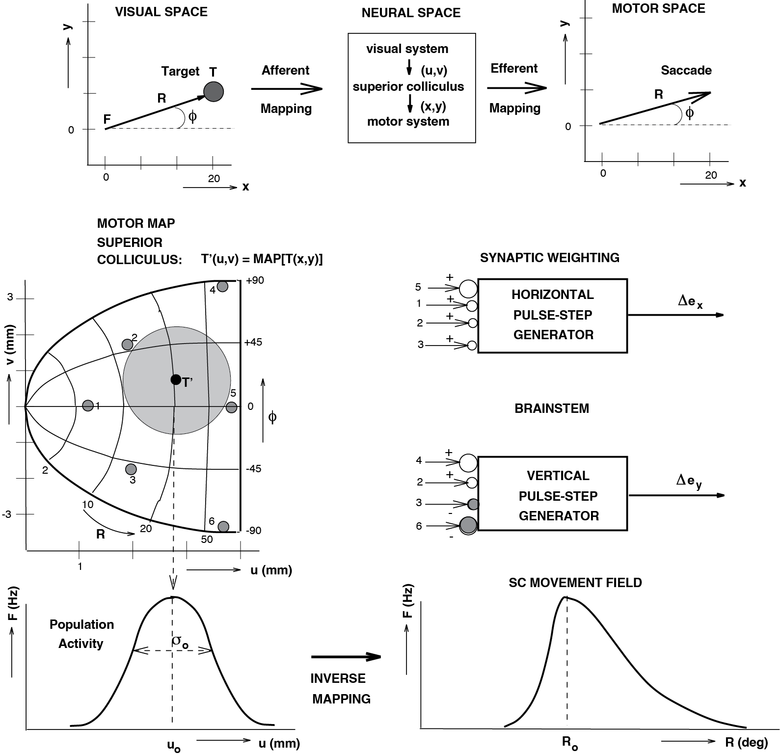
Fig. 68 Conceptual model of the mappings that take place between the early visual stage of the retina, and the final motor stage in the brainstem (top). Center: Complex-logarithmic motor map of the Superior Colliculus. \((u, v)\) anatomical coordinates; \((R, \phi)\) polar coordinates of saccade vector corresponding to site \((u, v)\) through Eq. {eq}`eqn_mapeqn5#
Mapping Principles#
Topographic map#
Most visual areas in the brain map the visual world in a topographic way: neighbouring locations in visual space activate neighbouring regions in the visual system. Each location can be described by coordinates. For the visual field, it is usually more convenient to use polar coordinates than simple Cartesian \((x,y)\) coordinates (Fig. 69A,B; see this polar-coordinate introduction if you want a refresher). In polar coordinates, a point is described by:
Eccentricity \(r\): radial distance from the centre
Direction \(\phi\): angular position
We can easily convert from one coordinate system to the other:
On the retina, eccentricity \(r\) is the distance from the fovea (the central region with highest cell density) to the point that is stimulated by a visual target. The neural map is not just a 1:1 copy of the visual field. There is a systematic transformation from visual coordinates to neural coordinates. As an example, we first look at how the visual world is mapped into the neural space of primary visual cortex (the retinotopic map). For that, we need a few basic organisation principles of the retina:
The cell density in the retina, \(d(r)\), decreases with increasing distance \(r\) from the fovea:
\(d = d(r).\)The receptive field of a sensory neuron describes the region of the visual field that influences its activity. Retinal ganglion cell receptive fields are roughly circularly symmetric, and experimental data show that their radius \(\sigma\) grows approximately linearly with eccentricity: \(\sigma \propto r.\)
A visual stimulus that is matched to receptive field size activates a roughly constant number of ganglion cells. The total number of stimulated cells is
\( N = \pi \sigma^2(r)\, d(r) \approx \text{constant} \quad (\text{about } N \approx 35).\)
Combining this with \(\sigma \propto r\) implies that
\(d(r) \sim \frac{1}{r^2}.\)
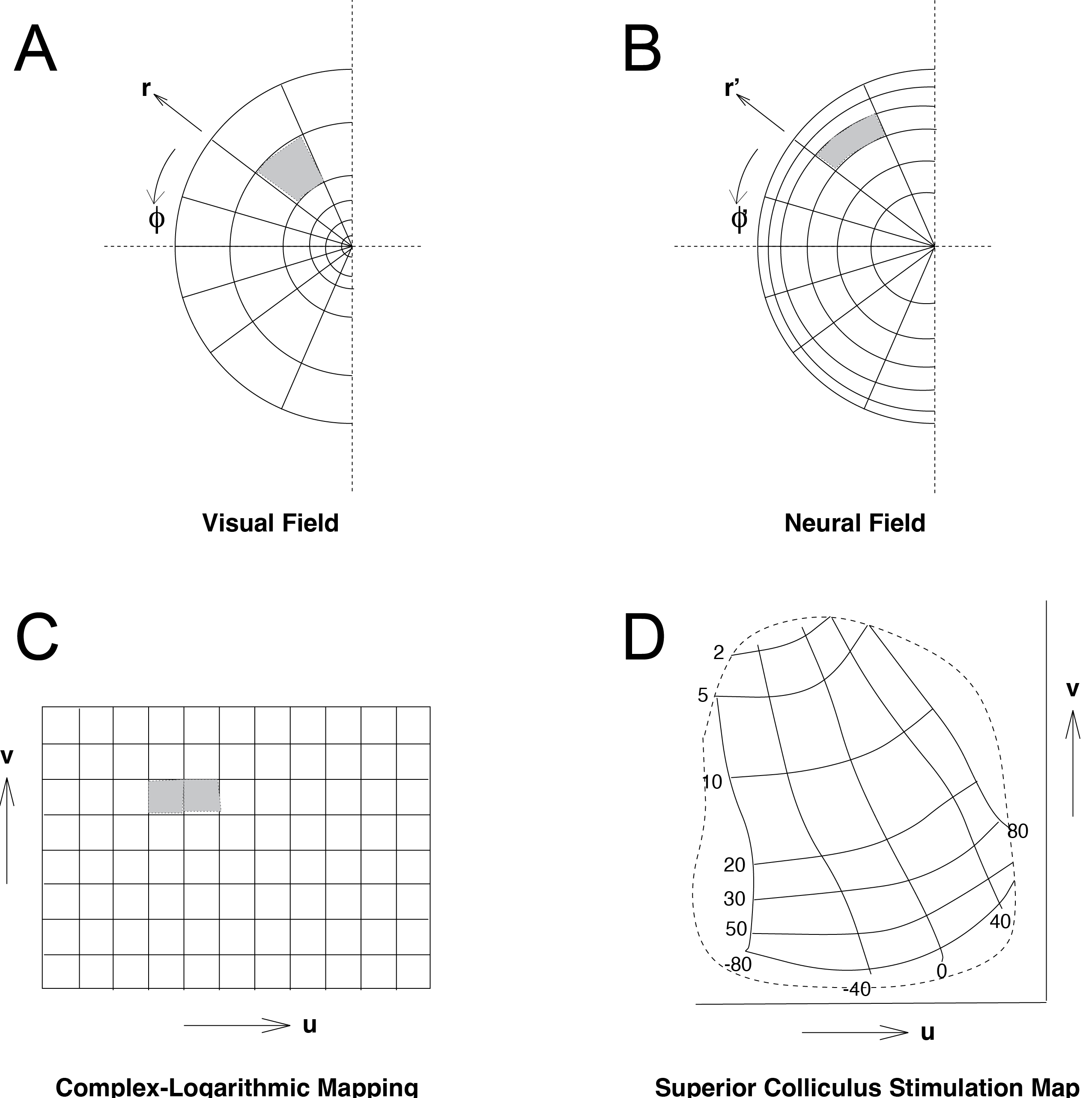
Fig. 69 Mapping of visual space onto neural space.#
Given this retinal organisation, what does the retinotopic map (the mapping from retina to visual cortex) look like? Suppose a small area \(\Delta A\) in the visual field is represented by \(\Delta N\) ganglion cells. Because each receptive field area \(A = \pi \sigma^2\) is represented by approximately the same number of cells \(N\), irrespective of \(r\), a relative change in receptive field area should correspond to the same relative change in cell number. Thus, the mapping must satisfy:
From Eq. (26) we define the local magnification factor \(M(r,\phi)\) as:
which relates small changes in the number of neurons to small changes in stimulated visual area. Taking the limit as \(\Delta N\) and \(\Delta A\) go to zero gives:
Solving this relationship by integration leads to the complex logarithmic map (Fig. 69C), which we will use below as the basis for understanding the motor map in the superior colliculus.
Cortical magnification factor#
We first consider the transformation from visual space to neural space in the primary visual cortex. This map is described by two cortical coordinates, \(X\) and \(Y\), which represent the horizontal and vertical positions on the cortical sheet (Fig. 70). Each cortical point corresponds to a location in the visual field specified by eccentricity \(r\) and direction \(\phi\). Thus, the map can be written as \(X(r,\phi)\) and \(Y(r,\phi)\).

Fig. 70 | Mapping of a patterned visual stimulus onto primary visual cortex (V1).#
A. A visual stimulus consisting of a rose pattern with three concentric rings at eccentricities of 1°, 2.3°, and 5.4°, and radial rays at cardinal and oblique directions (polar coordinates \(r,\phi\)).
B. Autoradiograph of primary visual cortex from the left hemisphere of a macaque monkey. The radioactive uptake pattern reflects the cortical activation produced by the visual stimulus similar to the one in panel A, revealing the topographic (retinotopic) layout of V1. Adapted from Tootell et al., 1982.
C. Mathematical logarithmic mapping that transforms visual polar coordinates \((r,\phi)\) into cortical coordinates \((X,Y)\), illustrating how eccentricity and direction in visual space are represented on the cortical surface.
To get a first approximation of this mapping, we make a simplifying assumption: for small regions of cortex, both the cortical coordinate \(X\) (considering radial directions) and the local magnification factor \(M(r)\) depend only on eccentricity. Under this assumption we obtain:
and the magnification factor is defined as:
Cortical Magnification Factor
The cortical magnification factor describes how much cortical surface area is devoted to processing a given amount of visual field. It is largest near the fovea, where visual acuity is highest, and decreases rapidly with eccentricity.
Formally, it is defined as:
\(M(r) = \frac{\text{mm of cortex}}{\text{deg of visual field}}\),
indicating how many millimeters of cortex represent one degree of visual angle at eccentricity \(r\). A high \(M(r)\) means that a small region of visual space is represented by a large area of cortex, enabling fine spatial resolution.
Physiological measurements in macaque visual cortex (e.g. Fig. 70B) show that the magnification factor decreases with eccentricity and is well approximated by
\(M(r) = \frac{\lambda}{r_0 + r}\),
with typical values \(\lambda \approx 12\) mm and \(r_0 \approx 1^\circ\). Integrating this expression gives, for \(r \gg r_0\):
Background - Derivation of the cortical magnification mapping
We start from the definition of the cortical magnification factor:
This yields the differential equation:
Step 1 — Integrate both sides
(see integration rules for rational functions)
Factor out the constant \(\lambda\):
Step 2 — Substitution
Let
Then
Substituting back:
Step 3 — Choose a reference point
Use the natural condition:
Then:
So:
Apply the log rule:
Final result
For large eccentricities \((r \gg r_0)\), this simplifies to:
This result shows how the logarithm arises naturally in cortical mapping: the visual-field coordinate \(r\) is transformed into a neural coordinate \(X\) by taking the natural logarithm. In primary visual cortex (V1), \(M(r)\) decreases approximately logarithmically with eccentricity, which causes equal steps in retinal eccentricity to appear as progressively smaller distances on the cortical surface. A key consequence of this transformation is that eccentric circles in the visual field (iso-\(r\) contours in Fig. 70A) become straight vertical lines in cortical space (iso-\(u\) lines in Fig. 70C): the entire 2D visual world (either in cartesian or in polar coordinates) is mapped onto a narrow, logarithmic ‘strip’ of neural tissue.
A similar derivation can be made for the directional component \(Y(r,\phi)\) using directional displacements \(dY\).
Background - complex logarithmic mapping
We have seen that transformation of retinal to cortical coordinates are achieved through logarithmic mapping and how complex number can represent two-dimensional vectors. Let’s combine these two concepts. We use the symbols \(u\) and \(v\) for the horizontal and vertical coordinates in the neural map (which we called \(X\) and \(Y\) before for the primary visual cortex), and \(x\) and \(y\) in the visual field. For the polar coordinates (eccentricity and direction/angle), we use \((r', \phi')\) and \((r, \phi)\) for the neural map and visual field, respectively. The complex-logarithmic mapping function is given by:
where the complex numbers \(\mathbf{z}\) and \(\mathbf{w}\) are defined as \(\mathbf{z}=x+i \cdot y=r \cdot e^{i\phi}\) and \(\mathbf{w}=u+i \cdot v=r' \cdot e^{i\phi'}\) (see Eq. (32)).
Complex numbers: See chapter Complex Numbers on complex numbers and the difference between polar and rectangular coordinates.
We also need to account for the magnification factor in the actual transformation from retinal to cortical coordinates. Thus, the neural mapping is of the form:
and so, \(u=B \cdot \ln{\sqrt{x^2+y^2}}=B \cdot \ln{(r)} \) and \(v=B \cdot \arctan{\frac{y}{x}}=B \cdot \phi \) (\(r\) and \(\phi\) in radians), with B the neural magnification factor, which indicates the amount of neural space (in mm) per radian angular change in the retina. This type of function has been proposed above to underlie the neural mapping from visual retinal space into visual cortical space. Note the singularity of this function at \(r = 0\), and note also the ‘forbidden regions’ given by \(|v| > B \cdot \frac{pi}{2}\). Thus, the entire 2D visual world (either in cartesian or in polar coordinates) is mapped onto a narrow, logarithmic ‘strip’ of neural tissue. You may verify that radiants (\(\phi\) = constant) are transformed into parallel horizontal lines, whereas circles (r = constant) transform into parallel vertical lines (see Fig. 69). For visual cortex, experiments have yielded a magnification factor of 1.4 mm/rad for both u and v coordinates (i.e. an isotropic mapping).
Sensorimotor mapping in the Superior Colliculus#
For the midbrain Superior Colliculus (SC), the afferent (sensory) mapping function (Fig. 71) is closely related to the complex-logarithmic mapping found in visual cortex.
Background – Differences between SC and V1 afferent mapping
But with two important modifications that reflect the SC’s role as a motor structure
The singularity at \(r = 0\) is removed by introducing a shift vector \(A = (A,0)\), because the SC does not represent the fovea directly.
The SC map is slightly anisotropic, meaning the horizontal and vertical magnification factors differ (\(B_u \neq B_v\)).

Fig. 71 | SC afferent and efferent mapping#
A. Visual space. Concentric rings and radial rays define polar coordinates. F = fixation; T = target; R = eccentricity; \(\phi\) = direction.
B. Neural (SC) space. Complex-logarithmic motor map with iso-\(R\) and iso-\(\phi\) contours. The transformation from visual to SC coordinates represents the afferent mapping.
C. Motor space. The saccade is ultimately executed by horizontal (x) and vertical (y) eye muscles. Mapping from SC to these motor commands corresponds to the efferent mapping.
Download Matlab code used to generate this figure, and to play around with target location
The experiment that motivated the quantitative description of this mapping is shown in Fig. 69 (bottom right). A remarkable observation is that a small electrical pulse (threshold ~10 µA) delivered through a microelectrode in the SC evokes a full, normal saccade. The size and direction of the evoked saccade depend only on the location of the electrode—not on the current amplitude or pulse frequency. By stimulating different SC sites, one obtains saccades with systematically varying amplitudes \(r\) and directions \(\phi\), which vary smoothly with the anatomical SC coordinates \((u,v)\). The resulting iso-amplitude (e.g., 2, 5, 10 … 50°) and iso-direction (e.g., −80, −40, 0, 40, 80°) contours form a topographic motor map that strongly resembles a complex-logarithmic transformation of visual space.
To describe these data, the following mapping function was proposed (Fig. 71):
where \(B_u\) and \(B_v\) are the horizontal and vertical magnification factors.
From nonlinear regression on microstimulation data, typical monkey values are:
Background – Complex-logarithmic formulation of SC mapping
The SC mapping can also be expressed compactly using complex numbers:
where
\(\mathbf{z} = R e^{i\phi}\) is the desired saccade vector,
\(\mathbf{w} = u + iv\) are SC coordinates,
\(\mathbf{A} = (A,0)\) removes the singularity at the origin,
\(\mathbf{B} = (B_u,B_v)\) captures the mapping anisotropy.
Properties of the SC motor map#
Conformal: local angles in visual space are preserved in neural space.
Inhomogeneous: small saccades (near the fovea) occupy more neural territory than large saccades.
Slightly anisotropic: horizontal and vertical scales differ, so shapes are stretched differently in \(u\) and \(v\).
The Superior Colliculus Motor Field#
When the saccadic system prepares an eye movement, activity must arise at the correct location in the SC motor map—the site whose coordinates encode the desired saccade vector. Microstimulation experiments (Fig. 69) demonstrate that activating a small cluster of neurons at a given map location is sufficient to produce a full, well‑formed saccade. But how does this relate to the activity of SC neurons during natural saccades?
To answer this, we introduce the concept of a movement field. A movement field is analogous to a receptive field in sensory systems: it describes the set of saccade vectors (amplitudes and directions) for which a given SC neuron becomes active. A neuron typically responds only when the planned saccade falls within a restricted region of \((R,\phi)\)-space.

Fig. 72 | Population activity and single-neuron movement fields in the Superior Colliculus.#
A. Population activity along the SC coordinate \(u\).
During a saccade, many SC neurons become active, forming a broad Gaussian-shaped population profile. Activity peaks at the location in the SC motor map that corresponds to the desired saccade vector.
B. Movement field of a single SC neuron along the amplitude dimension \(r\).
Each neuron responds to a range of saccade amplitudes, but this tuning is asymmetric (skewed), typically extending toward larger eccentricities. This reflects how individual movement fields relate to the overall population code.
Movement fields show several characteristic properties:
They are not rotationally symmetric.
Along the direction axis, responses tend to be roughly Gaussian, but along the amplitude axis movement fields are noticeably skewed, typically extending farther toward larger saccade amplitudes (see Fig. 72B).Their size scales with saccade amplitude.
Neurons coding small saccades have small movement fields, whereas those representing large saccades have much broader ones. In fact, movement field diameter increases approximately linearly with eccentricity—an interesting parallel to the increasing receptive field sizes in the retina described earlier.
These properties imply an important conclusion:
SC neurons are not sharply tuned to a single saccade vector. Instead, for any given saccade \((R_0, \phi_0)\), a population of neurons becomes active — specifically those whose movement fields include \((R_0, \phi_0)\). The center of this population corresponds closely to the location predicted by the SC mapping function (Eq. (28)).
This raises the key question developed in the next section: What determines the shape of this active population in SC coordinates, and how does that shape account for the observed movement field properties?
Population coding of saccades in the SC motor map#
A key insight into how the Superior Colliculus (SC) encodes saccades comes from examining movement fields after transforming them into SC coordinates using the mapping function (Eq. (28), Fig. 73).

Fig. 73 | Population activity in the SC motor map and its connection scheme to the brainstem.#
A. Population activity in the Superior Colliculus (SC).
A Gaussian-shaped activity profile is shown in \((u,v)\)-coordinates, centered at the map location encoding the desired saccade toward target T. The colored contours indicate firing-rate levels, peaking at the population center. Additional possible target locations (small grey numbered circles) illustrate how the same Gaussian activity pattern would translate across the motor map for different saccades.
B. Connection scheme and synaptic weighting.
For the grey-labeled SC sites shown in panel A, the corresponding synaptic projections to horizontal (top) and vertical (bottom) brainstem burst generators are illustrated. Cells 5 and 1 lie along the horizontal axis and therefore carry larger horizontal weights (open circles), whereas cells 2 and 3—located off-axis—contribute to both horizontal and vertical components. Conversely, cells 1 and 5 do not contribute to vertical saccades, while cells 4 and 6 do. Together, these fixed synaptic weight vectors implement the SC’s efferent (output) mapping.
When the skewed, amplitude-dependent movement fields of individual neurons are replotted in the \((u,v)\) coordinate system of the SC motor map, an important and surprising regularity emerges:
The remapped movement fields become invariant across the map.
Their size is approximately the same for neurons at all locations,
and the strong asymmetry observed in \((r, \phi)\)-space disappears.
In SC coordinates, the fields become rotation-symmetric
(see Fig. 68, bottom left).
This suggests the following interpretation:
Replotting a neuron’s movement field in SC coordinates effectively reveals the shape of the population activity that arises when a saccade is generated. If every site in the SC possesses a similar remapped movement field, then the population profile is identical for every saccade—its shape remains constant, and only its location shifts depending on the desired saccade vector (see Fig. 68, middle left).
Thus, the SC population activity is well described by a rotation-symmetric, shift-invariant, Gaussian function in \((u,v)\)-space:
where:
\(F_0\) is the peak firing rate,
\(\sigma_0\) is the spatial spread of the population,
\((u_0, v_0)\) is the center of the activity bump, given by the afferent mapping in Eq. (28).
Recordings from many SC neurons indicate typical parameters:
In summary, every saccade is encoded by the same Gaussian-shaped population, merely shifted across the SC surface depending on the saccade’s amplitude and direction. This forms the foundation for downstream decoding of saccade vectors in the brainstem.
Connection scheme of the Superior Colliculus with the brainstem#
Once a population of neurons in the Superior Colliculus (SC) is activated, the next question is how this activity is transformed into a saccade command for the brainstem pulse–step generators. Although many encoding schemes are theoretically possible, a remarkably simple and biologically plausible model captures the essence of how the SC specifies saccade direction and amplitude (see Fig. 68, center panel).
The model is based on three key principles:
Population coding (coarse coding):
Every neuron within the active Gaussian population contributes to the saccade—not just the neurons at the center of the bump.Firing-rate weighting:
Neurons that fire more strongly contribute more to the resulting saccade vector than weakly active neurons.Linear vector summation:
The final saccade vector arises from a weighted sum of all individual cell contributions.
Each neuron’s contribution is determined by two factors:
Its firing rate \(F_i\), which depends on the particular saccade being generated.
Its fixed synaptic projection \(\mathbf{W}_i\) to the horizontal and vertical pulse–step generators in the brainstem.
These synaptic weights depend only on the neuron’s location in the SC motor map and therefore constitute the efferent mapping of the SC.
Together, these principles lead to the following expression for the encoded saccade vector:
where:
\(\mathbf{z_0} = (\Delta x, \Delta y)\) is the desired 2D saccadic displacement,
\(F_i \in [0, F_0]\) is the firing rate of neuron \(i\) within the Gaussian population,
\(\mathbf{W}_i\) is the fixed synaptic weight vector from neuron \(i\) to the brainstem burst generators.
Conceptually, Eq. (31) states that each active SC neuron sends a small mini-vector to the brainstem. The size of this mini-vector is scaled by its firing rate, and the sum of all mini-vectors produces the correct saccade command.
Although it is analytically challenging to prove that this weighted-sum scheme yields the precise displacement needed to refixate a target, extensive computer simulations demonstrate that this population-vector mechanism accurately reproduces goal-directed saccades across the full range of amplitudes and directions.
Exercises#
Below you will find a set of exercises designed to deepen your understanding of afferent and efferent mapping, complex-logarithmic transformations, population coding, and anisotropy in the Superior Colliculus (SC). You can skip these.
Exercise 1 — Complex logarithmic mapping
The classical complex-log mapping has a singularity at \(z = 0\).
A more realistic mapping removes this singularity by introducing a shift vector:
a. Plot this modified complex-log map in 2D, similar to Fig. 69.
Show how radial lines and concentric circles are transformed.
b. Derive the inverse mapping:
Explain the steps:
use \(\mathbf{z} + \mathbf{a} = e^{\mathbf{w}}\), then subtract the shift vector.
Exercise 2 — Efferent mapping (inverse SC motor map)
The SC afferent map is given by Eq. (28).
Provide an expression for the inverse mapping (the efferent map):
which transforms SC coordinates \((u_0, v_0)\) back into the desired horizontal and vertical motor components \((\Delta x, \Delta y)\).
Hints:
Use the complex formulation (Eq. (29)):
\(\mathbf{z} = \mathbf{A}(e^{\mathbf{w}/\mathbf{B}} - 1)\).Extract \(R = |\mathbf{z}|\) and \(\phi = \arg(\mathbf{z})\).
Then convert \((R, \phi)\) to \((\Delta x, \Delta y)\).
Exercise 3 — Anisotropy and endpoint variability
Assume the brain selects the center \((u_0, v_0)\) of the Gaussian SC population, which determines the saccade vector \(\Delta e\).
Suppose this selection is noisy: repeated saccades to the same target yield population centers that lie within a small circular region in SC space.
a. Using Eq. (28), derive the corresponding distribution of saccade endpoints in \((\Delta x, \Delta y)\)-space.
Show that a circular region in SC coordinates becomes an elliptical region in motor space.
b. Explain why the ellipse axes are scaled by the magnification factors \(B_u\) and \(B_v\).
Conclude that the anisotropy \(B_u \neq B_v\) directly produces anisotropic endpoint scatter—even when the neural noise is isotropic.
Exercise 4 — Population coding and Gaussian invariance
Show that if the SC population activity is described by the Gaussian:
then for any saccade amplitude and direction the shape of the population is identical (same \(F_0\) and \(\sigma_0\)), and only the center \((u_0, v_0)\) shifts.
Explain why this property is essential for a stable population-vector readout.
Exercise 5 — Mini-vector summation (population decoding)
Using the population-decoding equation
simulate (or reason analytically) how the saccade vector changes when:
The Gaussian population is shifted slightly in \(u\).
The firing-rate gain \(F_0\) is doubled.
\(\sigma_0\) is widened (broader population).
Explain which changes affect saccade amplitude, saccade direction, or both.
Exercise 6 — Mapping distortions (conceptual)
Consider three targets at equal angular separation in visual space.
Using the SC map (Eq. (28)):
Plot their spacing in \((u,v)\)-coordinates.
Explain how the SC “allocates” neural space to different regions of the visual field.
Discuss why small saccades are encoded with finer neural precision than large ones.