Linear Systems

Introduction to linear systems

In this module, we will limit ourselves to the simplest class of systems:

• single input and output (see e.g. figure 1)

• time-invariant (the properties of the system do not change as a function of time (note, this is not self-evident, especially for biological systems! Think of ageing, fatigue, illness, etc.))

• causal (the value of the output depends only on values at the input in the past and present. Put a little neater: \(y(t) = F[x(s)] \textrm{for} s \leq t \) )

• linear systems.

Such systems have the following important property: \begin{definition}[superposition principle] A system is linear if the response to the weighted sum of any number of inputs equals the same weighted sum of the responses to the individual inputs.

\end{definition}

This property (requirement) is also called the Superposition Principle. This principle has some very important consequences, which we will discuss below.

Example

Suppose the response of a system to input signal \(x_1(t)\) is given by \(y_1(t)\), and the response to input \(x_2(t)\) is given by \(y_2(t)\). We now build a composite input, by taking a weighted sum: \(x(t) = a x_1(t)+ b x_2(t)\). Linearity of the system now requires that the response of the system to \(x(t)\) be given by: \(y(t) = a y_1(t)+ b y_2(t)\).

More generally:

(9)\[\textrm{if } x_i(t) \rightarrow y_i(t) \textrm{ then } \sum_{i=0}^{N} a_i x_i(t) \rightarrow \sum_{i=0}^{N} a_i y_i(t) \textrm{ for } a_i \in \mathbb{R}\]

The examples below show that linearity is not self-evident.

\begin{exercise}

Suppose a system multiplies an input signal by a certain factor, a, and then adds a fixed value, b:

\[y(t) = a \cdot x(t)+ b\]

In other words, the relationship between \(y(t)\) and \(x(t)\) describes a straight line. Now find out for which \(a\) and \(b\) this system is linear. (Hint: Apply the example above literally!) \end{exercise}

\begin{exercise} Suppose the input-output relationship of a system is given by:

\[y(t) = a \cdot x^2(t)+b\]

Show that this system can never be linear for \(a \neq 0\). (Hint: Do the same as in Exercise ex:straightline!) \end{exercise}

Impulse and step response

An important consequence of the Superposition Principle is the following: A linear system can be fully characterised by its impulse response.

\begin{definition}[impulse response] The impulse response of a system is the output signal as a function of time of that system when an impulse function is applied to the input. \end{definition}

An example can be seen in figure The impulse and the impulse response of an arbitrary linear system..

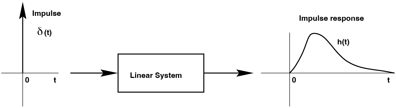
Fig. 8 The impulse and the impulse response of an arbitrary linear system.

The reason that the impulse plays such an important role for Linear Systems Theory lies in the property we encountered in eqn. eqn:impulse. The last line in that formula states that an arbitrary signal \(x(t)\) can be thought of as being made up of a series (i.e. a sum, or a superposition) of successive pulses, all of which have a different amplitude given by the value of the signal. This is qualitatively illustrated in figure Construction of a random signal as a sequence of weighted pulses.. Here we repeat that formula from eqn. eqn:impulse again for signal \(x(t)\):

\[x(\tau) = \int_{-\infty}^{+\infty} x(t) \cdot \delta (t-\tau) dt\]

but note that we may also write these as follows:

(10)\[x(t) = \int_{-\infty}^{+\infty} x(\tau) \cdot \delta (t-\tau) d \tau\]

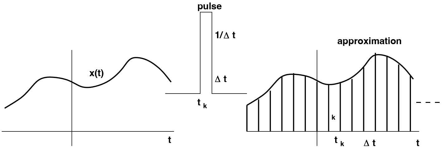
Fig. 9 Construction of a random signal as a sequence of weighted pulses.

In this last form, the whole signal \(x(t)\) is a sequence of individual pulses with height \(x(\tau)\), given at consecutive times (\(\tau\)). The superposition principle then says that the response of the linear system to such a weighted summed input is equal to the same weighted sum of individual impulse responses. So for a linear system, the response to any input signal can be calculated if we know the impulse response. This follows immediately from eqn. eqn:impulseend so that if the response to a single pulse \(\delta(t)\) is given by \(h(t)\), the response to the whole signal \(x(t)\) is given by:

(11)\[y(t) = \int_{-\infty}^{+\infty} x(\tau) \cdot h(t-\tau) d \tau\]

the same weighted sum of impulse responses, each given at times \(t_0\)! This formidable formula is also called the convolution integral.

Example: Step response

An important application of the above is the following. Suppose our input signal \(x(t)\) is a very simple one, namely a step, \(u(t)\) (Fig. The step function can be seen as a summation of successive pulses with weighting 1.). From \(t = 0\) it takes on the value 1, and before \(t = 0\) it was zero. So we can immediately substitute this simple input function into the convolution integral:

(12)\[y(t) = \int_{-\infty}^{+\infty} x(\tau) \cdot h(t-\tau) d\tau = \int_{0}^{+\infty} u(\tau) \cdot h(t-\tau) d\tau = \int_{0}^{t} 1 \cdot h(\tau) d\tau\]

where in the last step we have used the requirement that our system is causal (see a little later!).

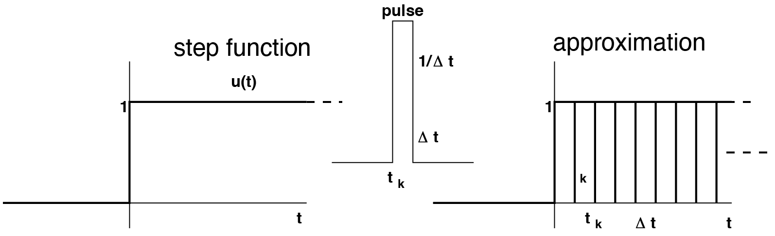
Fig. 10 The step function can be seen as a summation of successive pulses with weighting 1.

So, the step is actually nothing more than the cumulative area (the ‘integral’) of the impulse. After all: before \(t< 0\) the step is still zero, from \(t = 0\) it suddenly becomes 1 and remains that. It then follows that the response of a linear system to a step input, the Step Response (Fig. The step responses, s(t), or impulse response, h(t), is given.), is given by determining the cumulative area of the Impulse Response (i.e. the area as a function of time). Either:

\[y(t) = \int_{0}^{t} h(\tau) d\tau\]

Conversely, of course, the Impulse Response can also be determined from the Step Response by taking its derivative with respect to time:

\[h(t) = \frac{ds}{dt}\]

\begin{exercise} Some impulse responses (left) and step responses (right) are outlined in figure The step responses, s(t), or impulse response, h(t), is given.. Sketch the corresponding step or impulse for those systems. \end{exercise}

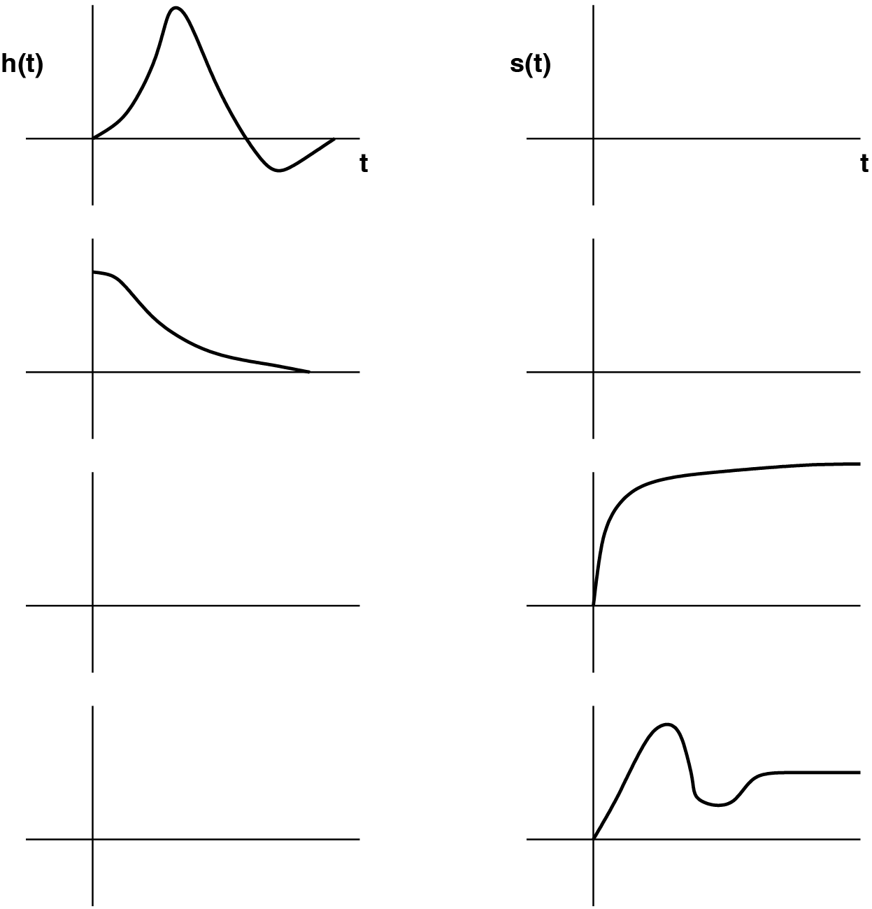
Fig. 11 The step responses, \(s(t)\), or impulse response, \(h(t)\), is given.

Response to a random stimulus for causal systems

Since we just saw that an arbitrary input signal can be described by a cumulative sum of successive weighted pulses (the areas of which are weighted by the value of the signal; see Fig. Construction of a random signal as a sequence of weighted pulses.), it follows from the superposition principle that the response to such a signal is given by taking the same weighted sum of pulse responses. So:

\[y(t) = \int_{-\infty}^{+\infty} x(\tau) \cdot h(t-\tau) d\tau\]

We now assume causality of the system. This means that the impulse response function can only be non-zero after the impulse has been given at time \(t\) (i.e. there can only be an effect after the cause). This means:

\[h(t) = 0 \textrm{ for } t<0\]

For the convolution integral, this means that:

\[h(t-\tau) = 0 \textrm{ for } t \geqslant \tau\]

In other words, to make the system causal, we write the convolution integral as follows:

\[y(t) = \int_{-\infty}^{t} x(\tau) \cdot h(t-\tau) d\tau\]

You will now see in the tutorial that this expression can be further modified into the more common form, commonly encountered in the literature as the convolution integral:

(13)\[y(t) = \int_{0}^{+\infty} x(t-\tau) \cdot h(\tau) d\tau\]

\begin{exercise} Try to understand eqn. eqn:convintegral by defining exactly what each quantity in the formula means. In short, state the conceptual meaning (in this equation) of \(t\), \(\tau\) , \(\tau = 0\), \(\tau = +\infty\), \(x(t-\tau)\), \(h(\tau)\) and \(\int\). (hint: why should \(h(\tau)\) be considered the memory of the linear system?) \end{exercise}

Although this formidable convolution integral in principle allows us to calculate the output on any input for any linear system, in practice it is often very difficult to calculate (analytically or numerically). Usually it must therefore be approximated on the computer.

\begin{exercise} For simple impulse responses and input signals it is sometimes possible to calculate the convolution integral. Let’s give that a try! Suppose that for a linear system the impulse response is given by \(h(\tau)=A \cdot exp (-a \cdot \tau)\). Then answer the following questions for this system:

[label=(\alph*)]

• Calculate and sketch the step response

• Suppose the input signal is given by a pulse of height B and duration T, and 0 elsewhere. calculate and outline the output of the system.

• Express the output of the system on the sum of the two inputs from (a) and (b) (\(B > 1\)).

\end{exercise}

Transfer (frequency) characteristics

The Fourier theorem (see section section:periodic) showed that ‘every periodic and transient signal can also be constructed from a sum of cosines, each with its own amplitude and phase. If so, according to the Superposition Principle, the response of a linear system should also be regarded as the summed response of “cosine responses”.

\begin{remark} An extremely important property of linear systems is that their output on a sinusoidal input always has the exact same frequency as the input. So only the amplitude and the phase of the cosine can be changed by a Linear System. \end{remark}

Why this property is a consequence of the Superposition Principle is by no means trivial: the convolution integral (Eqn. eqn:convintegral) should be able to answer this question. After all, it gives the output of a linear system on an arbitrary input, so also on a sine or cosine. Now suppose we have a sine wave as input signal:

\[x(t) = A \cdot \sin{(2 \pi f t +\Phi)} = A \cdot \sin{(\omega t +\Phi)}\]

and for simplicity let’s take \(A = 1\) and \( \Phi = 0\). According to Eqn. eqn:convintegral then holds for the output of the (arbitrary) linear system with impulse response \(h(t)\):

\[y(t) = \int_{0}^{+\infty} \sin{(\omega (t-\tau))} \cdot h(\tau) d\tau\]

This looks pretty hopeless at first glance, but let’s not despair. From our high school time we probably remember that (otherwise: see Binas or Wikipedia): \(sin(a - b) = sin(a)cos(b) - sin(b)cos(a)\). This is what we’re going to use here:

\[y(t) = \int_{0}^{+\infty} [\sin{(\omega t)}\cos{(\omega \tau)} - \sin{(\omega \tau)}\cos{(\omega t)}] \cdot h(\tau) d\tau\]

Now the next step: we have to realize here that the integration is taken over the variable \(\tau\) (the ‘memory time’), and that the ‘real time’, \(t\), can therefore be taken outside the integral with impunity (as if it were a constant):

\[y(t) = \sin{(\omega t)} \int_{0}^{+\infty} \cos{(\omega \tau)} \cdot h(\tau) d\tau - \cos{(\omega t)}\int_{0}^{+\infty} \sin{(\omega \tau)} \cdot h(\tau) d\tau\]

and now we realize that we cannot calculate the integrals, as long as we do not know exactly what kind of system we are dealing with. But be that as it may, and whatever system it is, the integral will simply produce something that no longer depends on \(\tau\). The only thing we can say about it is that the result of the integration will be a function of \(\omega\), and that it is different for the two integrals:

\[y(t) = \sin{(\omega t)} A(\omega) - \cos{(\omega t)} B (\omega)\]

in which:

\[A(\omega) \equiv \int_{0}^{+\infty} \cos{(\omega \tau)} \cdot h(\tau) d\tau \textrm{ and } B(\omega) \equiv \int_{0}^{+\infty} \sin{(\omega \tau)} \cdot h(\tau) d\tau\]

Now compare these last expressions with the Fourier series of expressions for the Fourier coefficients of \(a_n\) and \(b_n\) (eqn. eqn:analysiseqn). What you see here is the Fourier Transform of the Impulse Response. Finally, we dive back into our Binas booklet/Wikipedia/next exercise to see that this expression can also be rewritten as a single sine wave:

(14)\[y(t) = G(\omega) \sin{(\omega t + \Phi(\omega))}\]

\begin{exercise} Verify this last step, by expressing the functions \(G(\omega)\) and \(\Phi (\omega)\) in \(A(\omega)\) and \(B(\omega)\). \end{exercise}

Note that eqn. eqn:polarimpulseF tells us that the response of a linear system to a sinusoidal input with angular frequency \(\omega\) is given by a sine wave with the same angular frequency \(\omega\), but with a frequency-dependent amplitude, \(G(\omega)\) and phase, \(\Phi (\omega)\). By now looking at what the system does with the amplitude and phase of that sine/cosine for each sine/cosine component of the Fourier transform of the input signal, you can therefore obtain an alternative characterization from the system. Such an analysis therefore takes place in the frequency domain.

\begin{remark} In general, the amplitude and phase of the output are frequency dependent, and are completely determined by the properties of the linear system. \end{remark}

The behavior of the amplitude and phase as a function of the frequency is therefore characteristic of the specific linear system, and is also referred to as the **Transfer characteristic **of the system. The Gain of the system is defined as the ratio between output and input amplitude for each frequency: \(G(f)\), while the phase response is determined by taking the difference in phase between output and input cosine:\(\Phi (f)\). Gain and phase characteristic are usually plotted in a Bode plot (\(20 \log{(G)}\) and \(\Phi(f)\) as a function of \(\log{(f)}\). The ‘fingerprint’ that can then be seen in the frequency domain fully characterizes the linear system. Although usually only the amplitude characteristic is considered, actually both functions together determine the complete transfer characteristic. The transfer characteristic often enables us to understand the properties of a system at a glance. Therefore, such characteristics are used more than the impulse response (see above) in system analysis. Of course, there is an ‘unambiguous’ relationship between the two system representations, since both completely determine the behavior of the system. In view of the foregoing, it will be plausible that this relation is given by the Fourier transform. In other words:

\begin{remark} The Transfer Characteristic is the Fourier Transform of the Impulse Response. \end{remark}

• Fourier transform: \(h(\tau) \Rightarrow H(f)\), the spectrum (gain and phase)

• Inverse Fourier transform: \(H(f) \Rightarrow h(\tau)\)

Transfer characteristics of important linear systems

Important characteristics that are common in Linear Systems Theory (and in the models of biological systems) are:

• the Low-Pass (LP) characteristic: such a system passes low frequencies well, but stops the high frequencies.

• The High-Pass (HP) characteristic allows the high frequencies to pass well and stops slow changes in the signal.

• The Band-Pass (BP) characteristic allows only a specific band of frequencies to pass; frequencies that are higher or lower do not come through.

• The Band-Stop (BS) characteristic just stops all frequencies within a special band.

• The Time Delay (the ‘delay’): passes all frequencies equally well (‘All-Pass’), but with a fixed delay, \(\Delta T\): \(y(t) = x(t-\Delta T)\)

• The Integrator: integrates the input. Is an LP system.

• The Differentiator: differentiates the input (determines the derivative). Is HP.

Two simple linear systems are shown in Figs. Example of the Bode plot of a simple low-pass (LP) system: a resistor, R, in series with a capacitor, C. The output voltage is measured across the capacitor. High frequencies are passed through strongly attenuated and are 90 degrees out of phase, while low frequencies come through virtually unscathed and without delay. The impulse and step responses are also given. and Example of the Bode plot of a simple low-pass (LP) system: a resistor, R, in series with a capacitor, C. The output voltage is measured across the capacitor. High frequencies are passed through strongly attenuated and are 90 degrees out of phase, while low frequencies come through virtually unscathed and without delay. The impulse and step responses are also given., consisting of a resistor and a capacitor, which can have both a low-pass and a high-pass transfer characteristic.

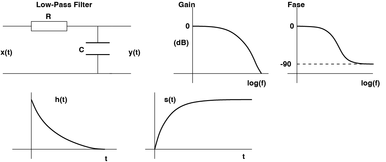
Fig. 12 Example of the Bode plot of a simple low-pass (LP) system: a resistor, R, in series with a capacitor, C. The output voltage is measured across the capacitor. High frequencies are passed through strongly attenuated and are 90 degrees out of phase, while low frequencies come through virtually unscathed and without delay. The impulse and step responses are also given.

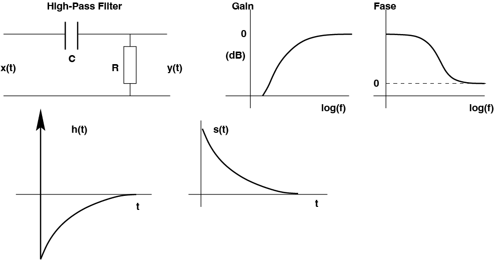
Fig. 13 Example of the Bode plot of a simple high-pass (HP) system: again the resistor, in series with a capacitor, with the output voltage now measured across the resistor. High frequencies are passed well without phase shift, while low frequencies are strongly attenuated. The impulse and step responses are also given.

There appears to be an important advantage to analyze systems in the frequency domain instead of in the time domain. The reason is that the relationship between input \(X(f)\), transfer characteristic \(H(f)\), and the output \(Y(f)\) in the frequency domain can be represented in the following simple way:

\[Y(f) = H(f) \cdot X(f)\]

In other words, to calculate the spectrum of the output, one only has to algebraically multiply the spectra of the transfer characteristic and the input signal frequency-wise. In practice, this turns out to be much simpler than calculating the response of the system in the time domain (which turns out to be a very laborious integration).

\begin{remark} Convention: Capital letters indicate that we work in the frequency domain [\(H(f)\), \(Y(f)\), \(X(f)\)]. Lowercase letters represent signals and characteristics in the time domain [\(h(\tau)\), \(x(t)\), \(y(t)\)] \end{remark}

Combination of linear systems

A direct consequence of this simple rule is that it becomes very easy to analyze arbitrary combinations of linear systems. In fact, a combination of linear systems also results in a linear system. The three combinations that are important in this course are:

• the series connection

• the parallel connection

• feedback (“feedback”). We will dwell on this form in particular, because it is important for the saccadic system.

The series circuit

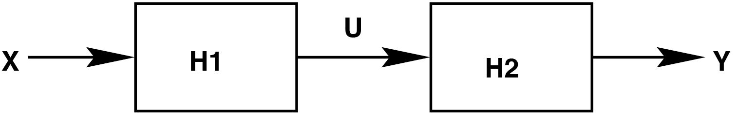
Fig. 14 A series circuit of two linear systems.

The first circuit we discuss is two systems in series (Fig. A series circuit of two linear systems.). To determine the total transfer of combined systems in general, it is useful to enter an auxiliary signal. In this case, we enter \(U\) as the output of system \(H_1\), which is serving as an input to system \(H_2\). Now verify, by applying the multiplication rule above, that the relationship between the final output \(Y\), and input \(X\) holds:

\[Y = H_1 \cdot H_2 \cdot X \Rightarrow H = H_1 \cdot H_2\]

\begin{exercise} Consider a Low-Pass and a High-Pass system with their characteristics (e.g. as above in Figs. Example of the Bode plot of a simple low-pass (LP) system: a resistor, R, in series with a capacitor, C. The output voltage is measured across the capacitor. High frequencies are passed through strongly attenuated and are 90 degrees out of phase, while low frequencies come through virtually unscathed and without delay. The impulse and step responses are also given. and Example of the Bode plot of a simple high-pass (HP) system: again the resistor, in series with a capacitor, with the output voltage now measured across the resistor. High frequencies are passed well without phase shift, while low frequencies are strongly attenuated. The impulse and step responses are also given.). What can you say about the total transfer if both systems are connected in series? Can you distinguish different cases? \end{exercise}

An example of serial system switching in a biological system, for example, is formed by the various sub-processes that make up our ear.

• \(H_1\) = Pinna and ear canal

• \(H_2\) = Middle ear bones

• \(H_3\) = Inner ear (cochlea)

The parallel circuit

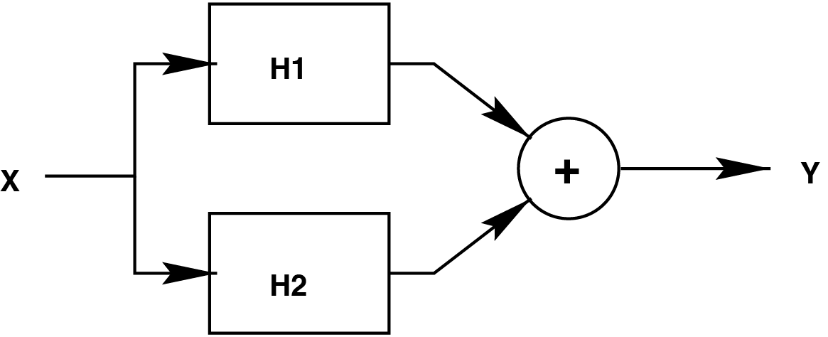
Fig. 15 A parallel circuit of two linear systems.

It is easy to see that in a parallel circuit the total transfer characteristic holds:

\[Y = (H_1 + H_2) \cdot X \Rightarrow H = H_1 \cdot H_2\]

In parallel circuits, the transfer functions of the different subsystems simply add up.

\begin{exercise} What can you say about the total transfer for a \(H_1 =\) Low-Pass system parallel to a \(H_2 =\) High-Pass system? \end{exercise}

Feedback

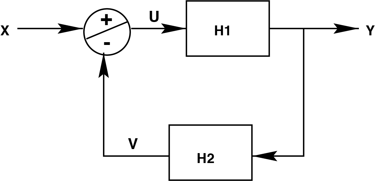
Fig. 16 Feedback with two linear systems.

To determine the total transfer of a feedback system (Fig. Feedback with two linear systems.) we introduce two auxiliary signals: \(U\) is the result of the addition/subtraction operation, \(V\) is the output of system \(H_2\).

• \(Y = H_1 \cdot U\)

• while \(U = X - V\)

• and \(V = H_2 \cdot Y\)

The total transfer of the system, \(\frac{Y}{X}\), is then (but check of course):

(15)\[\frac{Y}{X} \equiv H = \frac{H_1}{1+H_1 \cdot H_2}\]

Feedback is an essential aspect of more complex (especially biological) systems. So there will be a certain advantage to be gained with feedback. A first advantage can be seen if we can assume that (for a relevant frequency range) it holds that \(H_1(f) \cdot H_2(f ) \gg 1\). In that case eqn. eqn:feedbacktransfer will reduce to:

(16)\[H(f) = \frac{1}{H_2(f)}\]

The transfer has become independent of the system in the forward signal path. Here lies, among other things, the power of feedback, because if we for example have a system of which this so-called “forward gain” varies a lot or for example contains vulnerable components, feedback is sufficient to still get a reliable transfer.

Example: the smooth pursuit system

The smooth pursuit system serves to precisely follow a moving object in the outside world with the eyes. The input to this system is the speed of the moving object (e.g. a bird in the air, or the license plate of a car moving away) on the retina. This is also referred to as the retinal slip velocity. The aim of the system is to keep this slip speed as small as possible (preferably zero, because in that case the eye moves exactly as fast as the object). The output of the system is, of course, the speed of the moving eyes. Now note that this is a negative feedback system, the feedback of which is given ‘automatically’ by the eye’s own movement (see Fig. Simple model of the smooth pursuit system.).

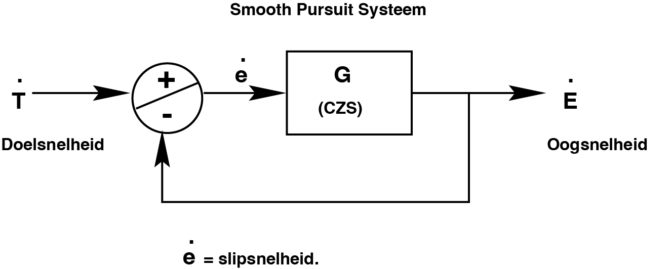
Fig. 17 Simple model of the smooth pursuit system.

Thus, the transfer of this system is given by:

\[\frac{\dot{E}}{\dot{T}} \equiv G_{tot} = \frac{G}{1+G}\]

Here \(G\) is the forward gain of the feedback system. You could see this as a process that takes place somewhere in the brain: the measured movement on the retina, \(\dot(e)\), is converted into a speed of the eye, \(\dot{E}\) after amplification with \(G\). This changes the difference in speeds between the target (\(\dot{T}\)) and the eye, i.e. the slip speed on the retina, a result of the feedback. The system tries to make \(\dot{E}\) and \(\dot{T}\) equal, so that \(\dot(e)=0\). To do this, the total transfer, \(G_{tot}\), must be close to 1 and for that the system gain, \(G\), should be large. \(G\) can be measured directly with the following experiment:

• The eye that sees the stimulus movement is temporarily paralyzed.

• The eye movement of the unparalyzed, but covered eye is measured.

\begin{exercise} Explain why we can directly measure the internal gain \(G\) of this system with this experiment (the gain \(G\) turns out to be about 20). \end{exercise}

Another advantage of feedback

From eqn. eqn:feedbacktransferreduced we see something else that could be seen as an advantage:

\begin{remark} In a feedback system with a large internal forward gain \(H_1(f)\) the total system does the inverse of \(H_2(f).\) \end{remark}

Summary

Summarizing:

[label=(\alph*)]

• Feedback stabilizes the system against external disturbances.

• It allows accurate transmission with a system consisting of unreliable (or diseased) elements.

• Feedback with a high forward gain (amplitude of H1 large) makes the response of a slow forward system fast.

• Note: Too much feedback (gain of H2(f ) also very high) can make the system unstable! (i.e. start to oscillate).

More information about the applications and backgrounds of the linear system theory can be found in the powerpoint files.

Exercises

\begin{exercise} Briefly explain whether \(y(t) = a \cdot x(t) + b\) is a linear system. \end{exercise}

\begin{exercise} Briefly explain whether \( y(t) = a \cdot x2(t) + b \cdot x(t)\) is a linear system. \end{exercise}

\begin{exercise} Briefly explain whether \( y(t) = a \cdot \frac{dx}{dt}\) (differentiation) is a linear system. \end{exercise}

\begin{exercise} Suppose that the visual system is a linear system that reacts to a retinal stimulus at position \(x(t)\) deg, with an eye-movement response to position \(y(t)\) deg. The response lasts \(D\) sec, and has a peak velocity of \(V\) deg/sec. Suppose that we scale the input with an arbitrary factor \(a\), so that \(x_2(t) = a \cdot x(t)\) What can you tell about the duration and peak velocity of this system’s output, \(y_2(t)\)? Sketch some stimulus-response pairs.

\end{exercise}

\begin{exercise} The pure Integrator (a concept that will come back when we discuss the oculomotor system!) is a system defined by the following input-output relation:

\[y(t) = \int_{0}^{t} x(\tau) d \tau\]

• Show that this is a linear system (test superposition!).

• what is the impulse response?

• What is the step response?

• Determine its amplitude and phase characteristics. Hint: what is the response of this system to \(x(t) = \sin{(\omega t)}\) ?

• Why do we call a low-pass filter a “leaky integrator”?

\end{exercise}

\begin{exercise} The pure differentiator is defined by input-output relation: \(y(t)=\frac{dx}{dt}\). Answer the same questions a to d as in the previous exercise. \end{exercise}

\begin{exercise} The pure time delay is given by the following input-output relation: \(y(t) = x(t-T)\) Same questions a-d as in Exercise 5.14. \end{exercise}