Reaction Times#
Learning Outcomes#
Learning Goals
Reaction times are a central tool in psychophysics and systems neuroscience.
The basic premise is simple but profound: neural processing takes time, and the timing of responses carries information about how the brain processes, evaluates, and acts on sensory input.
After completing this module, you will be able to:
explain what reaction times are and why they are informative
describe the characteristic distribution of reaction times and why it is skewed
explain why reaction times are stochastic rather than fixed
interpret reaction times as reflecting decision processes, not just sensory delays
describe the core assumptions and predictions of the LATER model
These learning outcomes connect directly to the course learning goals:
describe psychophysical methods and analyse psychophysical data
explain behaviour using simple neural and systems-level models
relate neural dynamics to perception and action
Optional Materials
Some sections include background boxes or optional mathematical detail.
These are not required for the exam, but they will help you connect this module to modelling, MATLAB exercises, and later topics (e.g. Bayesian inference, race models).
Background: Mental Chronometry#
Donders and “timing the mind”#
The Donders Institute is named after Franciscus Cornelis Donders, one of the first scientists to argue that mental operations are not instantaneous but take measurable time. In the mid-19th century, Donders introduced mental chronometry: the idea that the duration of internal cognitive processes can be inferred from reaction times. Donders proposed that a behavioural response could be decomposed into a sequence of processing stages, each contributing a delay:
sensory encoding (perception)
central processing (discrimination, choice)
motor execution
By comparing reaction times across different tasks, he introduced the subtraction method:
Simple reaction time: stimulus → response
Go / No-Go (discrimination): stimulus → decide whether to respond → response
Choice reaction time: stimulus → discriminate → select response → response
If these stages are arranged serially and add linearly (Fig. 77), then subtracting mean reaction times between tasks reveals the duration of individual mental operations. This logic still underlies much of modern neuroscience, from reaction-time experiments to fMRI contrasts.
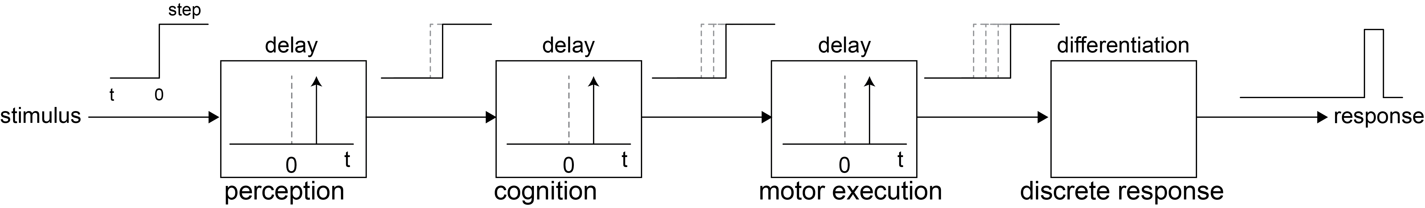
Fig. 77 | Mental chronometry#
A linear stage model of mental processing. If processing stages add linearly, their durations can be estimated using reaction-time differences (the subtraction method).
Background: The Stroop Task and Reaction Times
What is the Stroop task?
The Stroop task is a classic demonstration that perception, cognition, and action are not independent stages, but can interfere with each other. In a typical Stroop experiment, participants see words that name colours (e.g. GREEN, RED, BLUE), printed in coloured ink.
They are instructed to respond as quickly as possible to the ink colour, not the word itself.
Examples:
The word GREEN printed in green ink → congruent
The word GREEN printed in red ink → incongruent (Fig. 78)

Fig. 78 | The Stroop Task#
you have to indicate the colour or repeat the word.
What happens to reaction times?
Reaction times show a robust and highly reproducible effect:
Congruent trials → fastest reaction times
Neutral trials (e.g. coloured shapes or XXXX) → intermediate reaction times
Incongruent trials → slower reaction times and more errors
The increase in reaction time for incongruent trials is called the Stroop interference effect.
Why does this happen?
Reading words is an overlearned, automatic process, whereas naming ink colour is less automatic. On incongruent trials, two competing responses are activated:
the word meaning suggests one response (e.g. “green”)
the ink colour requires a different response (e.g. “red”)
Resolving this conflict requires additional central processing time:
suppression of the automatic word response
selection of the correct colour response
This extra processing time is directly visible as an increase in reaction time.
Why is the Stroop task important for mental chronometry?
The Stroop task shows that:
reaction times do not reflect simple sensory or motor delays
internal decision and conflict-resolution processes take measurable time
cognitive control can be quantified using reaction times
For Donders, this would correspond to adding an extra processing stage.
For modern models (such as LATER), Stroop interference can be interpreted as:
slower evidence accumulation
increased competition between decision processes
or a higher effective decision threshold
Thus, the Stroop task provides a clear demonstration that reaction time reflects decision-making, not just perception or movement.
Reaction time#
Reaction time (also called latency) is defined as the time interval between the onset of a stimulus and the onset of the corresponding response:
This definition is deliberately abstract. Reaction time is defined independently of:
the type of stimulus (e.g. sound, light, touch)
the type of response (e.g. saccade, button press, verbal response)
What matters is not what is sensed or how the response is executed, but when the decision to act is expressed in behaviour. This abstraction is precisely what makes reaction time such a powerful tool in neuroscience and psychophysics: it allows us to compare processing across sensory modalities, motor systems, and tasks using a single measurable variable.
Background: clarifications about reaction time
The definition of reaction time as
comes with several important caveats.
1. Reaction time is not the interval between stimulus offset and response onset
Reaction time is always defined relative to the onset of a stimulus, not its offset. Intervals measured from stimulus offset reflect different processes and are usually analysed separately.
2. Not all responses are stimulus-driven
Through the definition of reaction time, one can still formally determine reaction times for all responses. However, responses that are very early or very late are often generated by different mechanisms than the stimulus-driven decision process of interest. Examples include:
Predictive responses, where the participant anticipates the stimulus
Late responses, caused by inattentiveness, uncertainty, or secondary decision processes
Although these responses yield valid reaction-time values by definition, they typically follow a different statistical distribution and reflect different underlying neural mechanisms. For this reason, such trials are often analysed separately or excluded when the goal is to characterise stimulus-driven decision making.
3. Stimulus onset is not always well-defined
For brief, abrupt stimuli (e.g. a flashed light or click), stimulus onset is clear. For slowly emerging or natural stimuli (e.g. speech, motion ramps, or continuous sounds), onset may be ambiguous.
In such cases:
the definition of stimulus onset must be specified explicitly
reaction time may no longer be the most informative measure
4. Response onset must also be defined operationally
Responses are not instantaneous; they unfold over time. Therefore, response onset must be defined using a criterion, for example:
a velocity threshold for saccades
a force or displacement threshold for button presses
an acoustic level threshold for vocal responses
You have already encountered this in earlier modules, where saccade onset was defined using a velocity criterion (Assignment: The Linear Pulse-Step generator). Different onset criteria can shift measured reaction times systematically, so they must always be reported clearly.
Two Mysterious Properties of Reaction Times#
When reaction times are measured systematically, two striking and initially puzzling properties emerge:
Reaction times are surprisingly long
Reaction times are surprisingly variable
Both properties are clearly illustrated by saccadic eye movements (Fig. 79). We have seen in earlier modules that saccades are:
highly accurate (The Saccadic System - The Burst Generator)
extremely common (The Saccadic System - Pulse-Step Generator)
Humans make approximately two to three saccades per second, making saccades the most frequent voluntary movements we perform (far more frequent than, for example, heartbeats in rest, which is about 1 Hz (60 beats/minute)). This high frequency allows neuroscientists and psychophysicists to record thousands of saccades non-invasively in a single afternoon, providing a rich and precise dataset of behavioural responses generated by the nervous system.
Saccades are also extraordinarily fast movements (The Saccadic System - Pulse-Step Generator). They are often described as a masterpiece of biological engineering: a precisely programmed pattern of acceleration and deceleration that can last as little as 20–30 ms (Fig. 38c, e.g. Fig. 79), reaching peak velocities of up to 800 deg/s (Fig. 38d).
Paradoxically, saccades are also surprisingly slow. The saccadic reaction time — the interval between target onset and saccade onset — is typically around 200 ms, almost an order of magnitude longer than the movement itself. This is illustrated in Fig. 79, which shows saccades made toward bright visual step targets of 5 degrees (after [Corneil et al., 2002]). Despite the fact that:
the targets are very bright,
their location is fully predictable,
their onset is abrupt and unambiguous,
and the stimuli are identical across trials,
reaction times still vary widely. In this example, the earliest saccade begins at approximately 146 ms, whereas the latest saccade begins around 270 ms. Thus, even under optimal and highly controlled conditions, saccadic reaction times are both long and variable.

Fig. 79 | Saccadic Reaction Times#
Saccades have astoundingly long and variable reaction times, even for bright, high-contrast visual targets with an amplitude of 5 degrees. These saccades are from one participant in a study on audiovisual integration by [Corneil et al., 2002]. Arrows indicate the reaction time of the earliest and the last saccadic response. Also indicated are their durations.
Importantly, these properties are not a consequence of how reaction time is defined, nor are they due to experimental noise or poor measurement. They appear to be universal:
they occur for visual, auditory, and tactile stimuli
they occur for eye movements, hand movements, and verbal responses
they are observed across species, from frogs to humans
This universality strongly suggests that long and variable reaction times reflect something fundamental about how the nervous system operates. At first glance, these properties may seem like a nuisance or a limitation of biological systems. In this module, we will see the opposite: reaction-time variability is highly informative, and it provides a powerful window into how the brain makes decisions under uncertainty.
Reaction Time as Decision Time#
Reaction times are not long because of neuronal delays#
At first glance, long reaction times may seem to be an unavoidable consequence of neural transmission delays. After all, neural processing is not instantaneous:
action potentials propagate at finite speeds along axons,
each synapse introduces a delay,
sensory receptors and muscles require time to activate.
However, these factors cannot explain reaction times on the order of hundreds of milliseconds.
We can estimate the contribution of pure conduction and synaptic delays by considering the shortest functional pathway for visually guided saccades, which passes through the superior colliculus (The Saccadic System - Superior Colliculus). The superficial layers of the superior colliculus contain visually driven neurons that respond approximately 40 ms after stimulus onset (as shown by electrophysiological recordings, reflecting the pathway from retina → superior colliculus). Electrical stimulation of deeper collicular layers evokes saccades after roughly 20 ms, reflecting the pathway from superior colliculus → brainstem → eye muscles (Fig. 47). Thus, with both stages simply arranged in series, saccadic latencies would be expected to be around 60 ms. Yet this prediction is strikingly wrong.
As shown in Fig. 80, the average reaction time for saccades toward visual step targets is around 260 ms—more than four times longer than the minimum predicted by conduction delays alone.

Fig. 80 | Histogram of Saccadic Reaction Times#
Saccadic reaction times are long and highly variable, even for simple, bright visual targets.
Why are reaction times so long?#
The key insight is that reaction time is not dominated by neural transmission delays, but by central decision processes (Fig. 43). In natural behaviour, the brain is rarely deciding simply whether a stimulus exists or where it is. Instead, it must evaluate multiple questions in parallel:
what the stimulus is,
whether it is relevant,
which action is appropriate,
and whether it is better to act immediately or to wait.
These evaluations require time.
To support this, the nervous system contains parallel cortical and subcortical pathways that actively delay action while information is being integrated and evaluated. This cortical and basal-ganglia-mediated “procrastination” prevents premature responses and ensures that behaviour is flexible and adaptive, rather than merely fast.
For visually guided saccades, this organisation is particularly clear:
the superior colliculus can generate rapid, reflexive eye movements,
cortical areas such as FEF, LIP, and SEF analyse colour, form, motion, context, goals, and expectations,
tonic inhibition from brainstem structures (e.g. omnipause neurons) suppresses saccade initiation until a decision is resolved.
A conceptual shift#
These observations lead to a crucial shift in how reaction times should be interpreted:
Reaction time primarily reflects the time required to make a decision, not the time required to transmit signals.
In other words:
Key Insight
Reaction time is essentially decision time.
By studying reaction times across different tasks and conditions, we can infer how decisions are made.
Questions#
Knowledge Question - Why are reaction times long?
A bright visual target appears abruptly at a known location. Electrophysiological recordings show that:
visual responses in the superior colliculus occur after ~40 ms,
electrical stimulation of the same region can evoke a saccade after ~20 ms.
Yet, the average saccadic reaction time is around 250 ms.
Explain why saccadic reaction times are much longer than the sum of these neural delays.
In your answer, refer to the role of cortical processing and decision making.
Answer
Although neural conduction and synaptic delays contribute to reaction time, they account for only a small fraction of the observed saccadic latency. The shortest pathway from retina to eye muscles via the superior colliculus predicts saccades after roughly 60 ms, but actual reaction times are typically around 250 ms. The additional time reflects central decision-making processes. Before initiating a saccade, cortical and subcortical areas evaluate the stimulus, its relevance, and the appropriate action. During this evaluation, tonic inhibition prevents premature activation of the motor pathway. Thus, saccadic reaction time is dominated by the time needed to resolve a decision, not by the time required to transmit signals through the nervous system.
Insight Question - Why delay the response?
Why does the nervous system delay the initiation of a saccade even when the sensory signal is strong and unambiguous? Explain how this delay can be beneficial for behaviour.
Answer
Delaying saccade initiation allows the nervous system to integrate sensory information with context, goals, and expectations before acting. Even when a stimulus is strong and unambiguous, acting immediately could lead to inappropriate or suboptimal behaviour. By postponing action, cortical decision processes can suppress reflexive responses and select the most appropriate action at the right moment. This delay improves behavioural flexibility and accuracy, even though it increases reaction time. Therefore, long reaction times are not a limitation of the nervous system but a functional consequence of decision making under uncertainty.
Application Question - Colour in the SC
Does the superior colliculus encode information about stimulus colour? Explain your answer using the distinction between fast subcortical pathways and slower cortical decision processes.
Answer
The superior colliculus does not encode stimulus colour in a meaningful way for decision making. The superior colliculus is part of a fast, subcortical pathway specialised for detecting where a stimulus is and rapidly orienting the eyes toward it. Its visually driven neurons respond primarily to stimulus location, onset, and salience, not to detailed stimulus properties such as colour or form. Information about what a stimulus is — such as its colour — is processed in cortical visual pathways. These cortical areas evaluate stimulus identity, relevance, and context and then influence saccade initiation by modulating activity in the superior colliculus and brainstem through inhibitory and excitatory control. Thus, colour information affects saccadic reaction times indirectly, via slower cortical decision processes, rather than being encoded directly in the superior colliculus itself.
Advanced note: Colour signals in the superior colliculus
Neurophysiological studies in macaque monkeys have shown that neurons in the intermediate layers of the superior colliculus do respond to isoluminant colour stimuli, and that changes in colour saturation can modulate SC activity during detection tasks [White et al., 2009]. These responses are generally less selective and feature-rich than colour representations in cortex, but they indicate that colour information can be present subcortically and contribute to orienting decisions.
The Stochastic Nature of Reaction Times#
Skewed distributions#
A second striking property of reaction times is already visible in Fig. 80: reaction times are stochastic. Even under identical experimental conditions, reaction times vary substantially from trial to trial. Because saccades (and many other responses) can be measured thousands of times, we can determine the structure of this variability with high precision.
When reaction times are plotted as a histogram, a characteristic pattern emerges:
a clearly right-skewed distribution
a large number of medium-latency responses
a long tail of slower responses
Importantly, when reaction times are plotted directly in milliseconds, this skewness is always present.
A non-standard distribution#
This skewed distribution does not conform well to common statistical models:
it is not Gaussian
it does not fit Poisson, exponential, or gamma distributions
(cf. spike-count and interspike-interval distributions discussed earlier: The Neural Code, Fig. 26, Fig. 27)
Even more striking is its universality (again). Very similar reaction-time distributions are observed:
across species (from frogs to humans),
across effectors (eye movements, hand movements, speech),
across sensory modalities (vision, audition, touch).
Question: Normal Distribution?
Suppose you have collected a large set of reaction times from an experiment. How could you test whether the reaction-time distribution follows a normal (Gaussian) distribution?
Answer
You may know this from a course on Statistics.
One way to test whether reaction times follow a normal distribution is to use a Q–Q plot.
If the data are normally distributed, the points in a Q–Q plot should lie approximately on a straight line. Systematic deviations, especially in the tails, indicate departures from normality such as skewness.
A second approach is to use a statistical normality test, such as the Lilliefors test or the Kolmogorov–Smirnov (KS) test. These tests quantify whether the observed distribution differs significantly from a normal distribution with the same mean and variance.
For reaction times, both Q–Q plots and normality tests typically reveal strong deviations from normality, reflecting the characteristic right-skewed shape of reaction-time distributions.
In Matlab, using the KS-test:
[h,p] = kstest(zscore(rt)) % for reaction time
this should yield \(h = 1\), \(p\ll 0.05\), indicating that the null-hypothesis can be rejected, and that the data (and more extreme data) is very unlikely under the null-hypothesis that reaction times follow a Gaussian distribution.
Why this is puzzling—and important#
That reaction-time distributions are not Gaussian is inconvenient from a modelling perspective. That they are universal suggests something far more important: this variability reflects a fundamental property of neural decision processes, not measurement noise or experimental imperfections. It would be tempting to treat reaction time as the fundamental variable, since both stimulus onset and response onset are physically observable events. However, the systematic skewness and universality of reaction-time distributions raise a deeper question:
Are we actually measuring the right variable?
Crucially, this variability is not noise to be averaged away. Instead, it is the key phenomenon that reaction-time models aim to explain. Understanding the form of this variability will force us to rethink what reaction time represents — and will ultimately lead us to a more fundamental description of decision making.
The fundamental variable: promptness#
The systematic skewness of reaction-time distributions suggests that reaction time itself may not be the fundamental quantity generated by the nervous system. Instead, reaction time may be the observable consequence of an underlying process with different statistical properties. A useful way to explore this idea is to consider how decisions might be generated neurally.
From time to rate#
Suppose that, following stimulus onset, a neural decision process is initiated. This process evolves over time and continues until some criterion is reached, at which point a response is triggered. Crucially, imagine that this process proceeds at a certain rate, and that this rate varies from trial to trial. If the rate of this underlying process varies, then the time required to reach threshold will also vary. Because time and rate are reciprocally related, even modest variability in rate will produce strongly skewed variability in time.
This observation leads to a key idea: rather than analysing reaction time \(T\) directly, it may be more informative to analyse its inverse,
Promptness can be interpreted as a measure of how quickly a decision process unfolds.
Promptness distributions#
If variability originates in the rate of an underlying process, then plotting reaction times may obscure the true structure of that variability. To test this, we can examine the distribution of promptness instead of reaction time. When the inverse of reaction time is plotted as a histogram, a striking change occurs (Fig. 81). The distribution is no longer skewed. Instead, it appears approximately symmetric and bell-shaped. This suggests that promptness, rather than reaction time itself, may follow a Gaussian distribution.

Fig. 81 | Histogram of Saccadic Promptness#
The inverse of reaction time (promptness) shows an approximately symmetric, bell-shaped distribution. A Kolmogorov–Smirnov test does not reject the null hypothesis that promptness is normally distributed (P = 0.64). The black lines and squares denote a normal distribution with mean and standard deviation of the inverse of reaction times.
Why this matters#
If promptness is normally distributed, this has two important implications:
It greatly simplifies mathematical analysis, since Gaussian variability is well understood.
More importantly, it suggests that we may have identified a more fundamental variable — one that reflects the stochastic properties of the underlying decision process itself.
From this perspective, the skewed distribution of reaction times is not mysterious at all. It is simply the transformation of a symmetric distribution in rate into an asymmetric distribution in time. This insight sets the stage for formal decision models, such as the LATER model, which explicitly describe how variability in decision rate gives rise to the observed reaction-time distributions.
Insight: Why Gaussian distributions are special
A Gaussian distribution is often considered more fundamental not because nature “prefers” Gaussians, but because many different underlying processes naturally lead to Gaussian variability. In the context of reaction times and decision making, there are several complementary reasons.
1. The Central Limit Principle (why Gaussians arise so often)
If a variable is the sum of many small, independent contributions, its distribution tends toward a Gaussian, regardless of the distribution of each contribution. In neural systems:
decision-related activity reflects the combined influence of
many synaptic inputs,
many neurons,
many sources of noise,
each contribution is small and partially independent.
As a result, variability in an underlying decision variable (such as a rate or evidence signal) is naturally expected to be approximately Gaussian. This makes a Gaussian distribution a strong candidate for a primitive or generative variable.
2. Symmetry signals a “natural” variable
Reaction times are asymmetric (right-skewed). Promptness (1/T) is approximately symmetric.
This matters because:
asymmetry often indicates a transformation of a more basic quantity,
symmetry suggests we are closer to the variable the system actually controls.
In LATER:
the brain does not generate “time”
it generates a rate of rise of a decision signal
time is a derived outcome of that rate reaching threshold
A symmetric (Gaussian) distribution strongly suggests we have identified the right coordinate system for the problem.
3. Gaussian noise is the simplest kind of noise
From a modelling perspective, Gaussian variability is special because it:
is fully described by two parameters (mean and variance),
has no preferred direction (no skew),
maximizes entropy given fixed variance (i.e. is the least structured distribution possible).
This means:
if a system is noisy but has no reason to favour particular deviations,
Gaussian variability is the default expectation.
When promptness is Gaussian, it suggests the system is not fine-tuned or artificial, but governed by generic stochastic principles.
4. Linear dynamics + Gaussian variability = Gaussian outcomes
In the LATER model:
the decision signal evolves linearly,
the variability enters through the rate,
if that rate is Gaussian, the mathematics remains simple and transparent.
This is important because:
linear + Gaussian systems are analytically tractable,
deviations from Gaussianity often signal additional mechanisms.
The success of Gaussian promptness implies that no extra machinery is needed to explain the data.
Reciprobit plots: a graphical representation of reaction-time distributions#
So far, we have seen that reaction times are skewed, whereas their inverse (promptness) appears to be approximately normally distributed. The next step is to find a clear and informative way to visualise this regularity.

Fig. 82 | Reciprobit plots#
a. Cumulative probability as a function of reciprocal reaction time (promptness).
b. The same cumulative probability plotted on a probit (Gaussian) scale, yielding a reciprobit plot.
Dots indicate individual responses; red circles indicate quantiles.
In panel b, the best-fitting regression line is shown in red, demonstrating the approximately linear relationship.
From histogram to cumulative distribution#
We start by converting the reaction-time histogram into a cumulative distribution function (CDF) (Fig. 82a). The CDF shows, for each value of promptness, the proportion of responses that are slower than that value.
Cumulative distributions are mathematically better behaved than histograms:
they are less sensitive to binning choices,
they emphasise the overall structure of the data,
and they are well suited for testing distributional assumptions.
The probit scale#
Next, we transform the vertical (probability) axis using a probit scale (Fig. 82b). A probit scale represents the inverse cumulative distribution function of a standard normal distribution. In other words, probabilities are mapped onto the z-scores of a Gaussian distribution.
This idea could be familiar from Statistics 1:
plotting data on a probit scale is closely related to a Q–Q plot
if data are normally distributed, the transformed points fall on a straight line
systematic deviations indicate departures from normality (e.g. skewness or heavy tails)
Thus, a probit plot provides a visual test for Gaussianity.
The reciprobit transformation#
Combining two transformations reveals a striking regularity:
take the reciprocal of reaction time: \(\frac{1}{T}\) (promptness)
plot the cumulative distribution on a probit (Gaussian) scale
Because this combines a reciprocal transformation on the horizontal axis with a probit transformation on the vertical axis, the resulting graph is called a reciprobit plot. The result is shown in Fig. 82b. Over most of the distribution, the data fall remarkably close to a straight line.
This implies that:
promptness is normally distributed
reaction times follow a recinormal distribution
Why reciprobit plots are powerful#
A straight line can be described by only two parameters:
a slope
an intercept
Remarkably, this means that under most conditions, reaction-time behaviour can be characterised by just a small number of parameters, despite the apparent complexity and variability of the raw data. In the next section, we will introduce a formal model that assigns a neural interpretation to these parameters.
Advanced: Early responses and multiple mechanisms
The reciprobit plot shown here focuses on the main part of the distribution. In very large datasets, a small number of very early responses can sometimes be observed, which form a second, shallower line. A plausible interpretation—consistent with the idea of cortical “procrastination”—is that:
the main distribution reflects decision processes at higher cortical levels
early responses arise from lower-level pathways that occasionally escape tonic inhibition, particularly under urgency, distraction, or impaired cortical control
Such early responses are often more error-prone and become more frequent in demanding or pathological conditions. Such early responses could also be highly cognitive, predictive responses.
Universality of the reciprobit law#
This empirical regularity is not limited to one task or response type. Reciprobit plots reveal similar linear structure across:
saccadic eye movements
manual responses
visual, auditory, and tactile stimuli
humans and other animals
This universality strongly suggests that reciprobit structure reflects a general principle of neural decision making, rather than a task-specific artefact.
An Empirical Model: LATER#
Core idea#
There is clear empirical value in being able to describe complex reaction-time data with only a small number of parameters. From a scientific perspective, however, it is even more satisfying to have a mechanistic model that explains why such simple regularities arise. Earlier, we saw that reaction times become highly regular when we analyse their reciprocal (promptness). This observation naturally suggests that reaction time is not generated directly, but instead reflects the outcome of an underlying process that evolves at a certain rate. The simplest model that captures this idea is the LATER model, which stands for Linear Approach to Threshold with Ergodic Rate — a name that also alludes to the idea of neural procrastination.
The LATER mechanism#
In the LATER model, a decision is represented by a single internal signal:
the signal starts at an initial level \(S_0\),
after stimulus onset, it rises linearly toward a threshold \(S_T\),
the slope (rate of rise) \(r\) varies randomly from trial to trial,
when the signal reaches threshold, a response is triggered.
The reaction time \(T\) on a given trial is therefore:
Crucially, the rate \(r\) is assumed to be normally distributed across trials, with mean \(\mu\) and variance \(\sigma^2\).As a direct consequence, the inverse of reaction time, \(\frac{1}{T}\), is also normally distributed. This single assumption immediately explains:
the skewed shape of reaction-time distributions,
the linear structure observed in reciprobit plots.

Fig. 83 | The LATER model#
A decision signal starts at level \(S_0\) and rises linearly toward a threshold \(S_T = S_0 + \theta\). On each trial, the rate of rise \(r\) is drawn from a Gaussian distribution with mean \(\mu\) and variance \(\sigma^2\). When the signal reaches threshold, the response is initiated. Variability in \(r\) produces a skewed distribution of reaction times.
Why LATER works#
The power of the LATER model lies in its simplicity. With only a small number of parameters, it captures the essential structure of reaction-time data across tasks, effectors, and species Empirically, the fact that reciprocal reaction times are normally distributed means that entire datasets can be summarised by just two parameters. Mechanistically, LATER provides a concrete neural interpretation of these parameters by linking them to a decision signal that accumulates toward threshold.
Key parameters and their interpretation#
The behaviour of the LATER system is governed by a few interpretable parameters:
Starting level (\(S_0\)) Reflects prior probability or expectation
Threshold (\(S_T\)) Reflects urgency or caution (how much evidence is required before acting)
Mean rate (\(\mu\)) Reflects the quality or strength of sensory evidence
Variance of the rate (\(\sigma^2\)) Determines trial-to-trial variability
One of the strengths of the LATER model is that its parameters map directly and predictably onto features of reciprobit plots. This makes it possible to infer properties of the underlying decision process simply by inspecting how reaction-time distributions change across conditions.
Swivels, shifts, and slopes#
Changes in the LATER parameters produce characteristic transformations of the reciprobit plot (Fig. 84):
Changing the starting level \(S_0\) or the threshold \(S_T\)
causes the reciprobit plot to swivel around a fixed intercept on the infinite-time axis.
Functionally, this reflects changes in prior expectation or urgency.Changing the mean rate of rise \(\mu\)
produces a horizontal, self-parallel shift of the reciprobit plot.
This corresponds to changes in the strength or quality of sensory evidence.Changing the variance of the rate \(\sigma^2\)
alters the slope of the reciprobit plot without changing the median reaction time.
Greater variability in rate produces shallower slopes.
These transformations are illustrated schematically in Fig. 84.
How many parameters does LATER really have?#
At first sight, the LATER model appears to contain four free parameters:
\(S_0\), \(S_T\), \(\mu\), and \(\sigma^2\).
In reality, the system has only two independent degrees of freedom:
only the difference between starting level and threshold matters
\( \Delta S = S_T - S_0\)the absolute scale of the decision signal is arbitrary
If \(\Delta S\), \(\mu\), and \(\sigma\) are all multiplied by the same factor, the predicted behaviour is unchanged. Moreover, altering \(\Delta S\) is mathematically equivalent to jointly altering \(\mu\) and \(\sigma\). For this reason, reaction-time behaviour is typically characterised empirically by just two parameters, usually taken as:
the mean of the reciprocal reaction times
the slope of the reciprobit plot
Fixed delays and practical modelling#
The LATER model deliberately ignores fixed delays that are unavoidable in real sensorimotor systems, such as:
receptor transduction,
synaptic delays,
axonal conduction,
muscle activation.
For visually guided saccades, these fixed delays are typically estimated to be around 50–60 ms.Importantly, adding a fixed delay of this magnitude has little effect on the linearity of reciprobit plots. For many purposes — such as behavioural characterisation or clinical assessment — this delay can therefore be safely ignored. In more complex paradigms (e.g. countermanding or task switching), fixed delays are usually included explicitly in the model.
Empirical parameterisation#
When fixed delays are ignored, reaction-time data are often described using empirical parameters derived directly from the reciprobit plot:
the intercept corresponds to the reciprocal of the median reaction time
the slope reflects variability in the underlying decision rate
Although these empirical parameters differ slightly from the true underlying model parameters, this distinction is unimportant for most practical applications. What matters is that a complex and noisy behavioural dataset can be captured accurately with just two numbers.

Fig. 84 | Relation between LATER parameters and reciprobit plots#
Top: changing the threshold causes the reciprobit plot to swivel around the infinite-time intercept.
Middle: changing the mean rate of rise produces a horizontal, self-parallel shift.
Bottom: changing the variance of the rate alters the slope without affecting the median.
Conceptual takeaway#
The LATER model provides a direct link between:
behavioural data (reaction times),
graphical structure (reciprobit plots),
and underlying decision mechanisms.
This tight correspondence is what makes reaction-time analysis such a powerful tool for studying decision making in the nervous system.
Other phenomena and models#
The LATER model provides a compact and powerful framework for understanding reaction-time distributions, but it is not the only model of decision making. Other widely used approaches include diffusion and accumulation models, in which evidence evolves as a noisy random walk rather than at a constant rate. These models are especially useful for describing tasks near sensory threshold and are discussed in more advanced courses. In addition, reaction-time data often contain features that go beyond the main distribution discussed here. Examples include:
very early (“maverick”) responses, which may reflect fast subcortical pathways or lapses of cortical inhibition,
multiple response components, indicating parallel decision mechanisms,
and changes in distribution shape under urgency, distraction, or neurological impairment.
Such phenomena can be accommodated within extended versions of the LATER framework, as well as by alternative models. In this module, we focus on LATER because it captures the essential structure of reaction-time behaviour with minimal assumptions and provides a clear bridge between empirical data and neural decision processes.
Optional Reading#
More information can be found in:
[Noorani and Carpenter, 2016]: a tutorial on the later model
[Roelofs, 2018]: Donders and reaction times
Follow-up#
In the next module (Assignment: Reaction Times) you will be doing your own reaction-time experiment, analysing this with a reciprobit plot, and interpreting this in terms of the LATER model.