Assignment: The Linear Pulse-Step generator#
Learning Goals#
In this computer exercise we will investigate the main properties of the saccade model by means of numerical simulations with Simulink (a graphical simulation package that runs under Matlab). By interactively changing the parameters in the model, we will gain a further understanding of:
some elementary concepts of the systems-theoretical approach: linearity, nonlinearity, feedback, ….
the role of different brainstem nuclei in saccade generation.
the effect on saccades of specific brainstem lesions.
Simulink#
Some remarks concerning Simulink:
After turning on the computer, double-click on the MATLAB icon, and wait until the command screen appears.
Activate the command screen (e.g. by left-clicking the mouse once inside the window) and type: \mcode{simulink}
You will now see a Simulink Library window and an Untitled window. Click on the File option in this latter window, and open \mcode{pulsestep.mdl} in the directory where you stored this file (from Brightspace).
Alternatively, open \mcode{saccade.mdl}. In the exercises, we will first start with the \mcode{pulsestep.mdl} version, which is a simpler model version of the final part of this model.
You can run either model simulation by clicking on the simulation option in the Model window, and subsequently on start. After choosing the simulation option, you may change the run-time simulation parameters (e.g. the simulation time, which is set at a default value of 0.5 sec).
By left-double-clicking the mouse on one of the coloured model’s boxes (see the exercises), a dialog window will open, in which the relevant numerical values are given. You may change these values and study the effect of these changes on the simulation results. Always ensure that you provide your numerical value in the required units (degrees, seconds, or milliseconds).
You may want to add a new display to your simulation, e.g. if you want to view the activity patterns of the OPNs or of the LLBNs in the model. In that case, you will have to carry out the following steps:
Open the sinks icon in the Library window, and drag one of the display icons (e.g. XY-graph or scope-graph (=YT)) to your model window.
Put the graphical tool close to the site where you need it.
You can then make a connection between the new display and the model, by pressing the left mouse button at the input site of the new display and, while keeping the mouse button pressed, moving the mouse toward the selected signal line of the model (not for the ‘cross hair’ to appear). Release the mouse button. You will now have established a connection.
Finally, you need to set the display parameters of the graphics box: double-click on the box (you will now see the display window), and click on the parameter setting of the scale.
You can remove the display box by clicking on the x in the top-right corner of the display window.
If you want to rerun the model with its default parameters, first close Simulink (click on the top-right x of the model window) (you may either keep or not keep your own settings on the main directory, by saving the model on your own name) and rerun Simulink in the command shell.
To create a figure of a Scope in a Word-document, you can copy (command-C (Mac OS) or control-C (Windows)) when the Scope is selected, and paste this into the Word-document.
Computer exercises with the linear PulseStep generator model#
To gain more insight into the concept of Pulse-Step Generation, and also to get more acquainted with the ideas behind Linear System’s Theory, a simple model of the so-called ‘Final Common Pathway’ of the oculomotor system (Fig. Model of the Final Common Pathway of the Oculomotor System. For saccades, this embodies the Pulse-Step Generator. The output of this pathway (i.e. eye position) is subsequently fed through an Inverse Model of the Plant, to enable a reconstruction of the motoneuron signal (see also Figs. {ref}`fig:omnreconstruction) is also available under Simulink as file \mcode{pulsestep.mdl} (Figs. fig:psgsimulink and fig:psgscope). This simulation model (compare it to the final part of the \mcode{saccade.mdl} model), allows you to interactively set parameters of:
The saccadic burst from the EBNs/IBNs (this is simply modeled as a pulse, having a height, \(P\), and duration \(D\).
The neural integrator: setting its gain to zero mimics total loss of the integrator, whereas a gain of one means normal operation.
The direct path: feeds the pulse directly to the oculomotor neurons. When its gain is set to zero, you actually simulate the effect of a Step input to the OMNs.
The Plant, with its two time constants, \(T_1\) and \(T_2\)
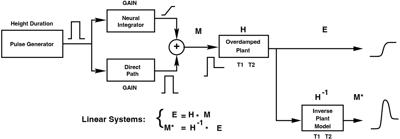
Fig. 49 Model of the Final Common Pathway of the Oculomotor System. For saccades, this embodies the Pulse-Step Generator. The output of this pathway (i.e. eye position) is subsequently fed through an Inverse Model of the Plant, to enable a reconstruction of the motoneuron signal (see also Figs. {ref}`fig:omnreconstruction#
```{figure images/simulink_pulsestep.png :name: fig:psgsimulink PulseStep Simulink Model. Compare to Fig. {ref}fig:psgmodel
```{figure` images/simulink_scopes.png
:name: fig:psgscope
Scopes in the PulseStep Model.
\begin{exercise}[Amplitude] How do you determine the amplitude of a saccade? \end{exercise}
\begin{exercise}[Parameters] First play with this model by changing the parameters of:
[label=(\alph*)]
the Burst (Burst Generator: Pulse Duration and Pulse Height)
the Neural Integrator (Integrator Gain)
the Forward Gain (Direct Path:Gain)
the Oculomotor Plant (Long Time Constant [T1] and Short Time Constant [T2])
Every time you change one parameter, make sure that the others are at their default value. Note what happens with each change in parameters. For example, if burst height changes (e.g. from 700 spikes/s to 300 spikes/s):
how large is saccade amplitude?
What is peak velocity?
What is saccade duration?
how did the pulse-step change (if any)?
\end{exercise}
\begin{exercise}[Linearity] Verify that the model is linear.
Hint: what is a linear system? A system that obeys the superposition principle (Def. def:superpositionprinciple). This theoretically means that you have to verify for all signals \(x\) and all weights \(a\) at all times \(t\), whether this holds. You will not have to do that.
You have to verify that the saccades (= the output signal) behave in a linear fashion for five heights of the burst (= the input signal; 167, 333, 500, 667 and 833 spikes/s; see also Exc. exc:psgparameters). Do so by \mcode{plot}ting relevant saccade parameters as a function of burst height (label the axes). Briefly explain (see also: (see Eqn. eqn:superpositionprinciple and exc:linearoculomotorsystem).
\end{exercise}
\begin{exercise}[Step response] Determine the Step response of the oculomotor plant.
How can you achieve this (which parameter of which block should be set to 0)?
What do you see (e.g. amplitude, velocity)? Check all signals in the Scopes and compare.
\end{exercise}
\begin{exercise}[Pulse-Step mismatch - Pulse Gain] Start with the default model parameters. Vary the strength of the Forward Gain (Direct Path) in the PulseStep model (from the default 0.15 to 0.05 and 0.25).
[label=(\alph*)]
We first concentrate on 20-deg saccades only. How can you make sure a 20-deg saccade is made? See (or revisit) your answers to Exercise exc:psgparameters and exc:psglinearity.
Describe the effect of these changes on the saccade.
Briefly explain.
Do the same effects also occur for saccades of different amplitudes (10, 25, 35 deg)?
\end{exercise}
\begin{exercise}[Pulse-Step mismatch - Oculomotor Plant] Again keep your default parameter set. Now only vary the long time constant of the plant, \(T_1\) (from the default 0.15 to 0.05 and 0.25).
[label=\alph*)]
Describe the effects on the saccade, and explain.
What do you conclude when you combine these effects with the previous exercise?
Test your hypothesis by introducing variations in both parameters, such that the saccade is unaffected (\mcode{plot}).
Does your parameter choice depend on the saccade amplitude?
\end{exercise}
\begin{exercise}[Pulse-Step mismatch - The Neural Position Integrator] By changing the gain of the Neural Integrator between 0 and 1, you may study the effects of lesions to the neural integrators on the saccades (for values of 0.1, 0.5, and 0.8 and for the rest keep your default parameter set).
[label=\alph*)]
Describe these effects, and explain.
What do you conclude when you combine these effects with the previous exercise?
Test your hypothesis by introducing variations in both parameters (Gain and T1), such that the saccade is unaffected (\mcode{plot}).
\end{exercise}
\begin{exercise}[Pulse-Step reconstruction] An additional feature of this simple simulation model is the possibility to reconstruct the actual net motoneuron input to the plant, on the basis of the (simulated) eye position signal. To that means, an inverse model of the plant is incorporated (see Fig. Model of the Final Common Pathway of the Oculomotor System. For saccades, this embodies the Pulse-Step Generator. The output of this pathway (i.e. eye position) is subsequently fed through an Inverse Model of the Plant, to enable a reconstruction of the motoneuron signal (see also Figs. {ref}`fig:omnreconstruction). Simulate the model with its default parameter set and note (\mcode{plot}) the (quite reasonable) resemblance between the reconstructed OMN input and the original Pulse-Step input. \end{exercise}
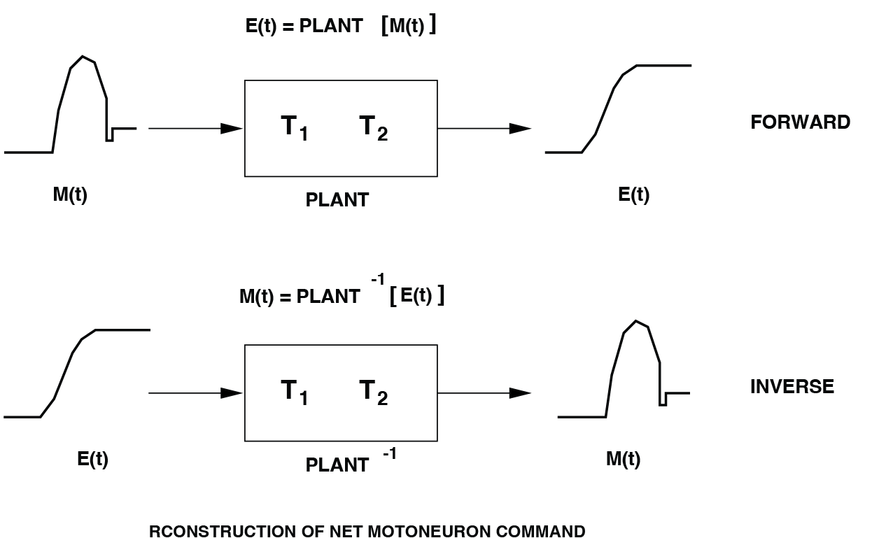
Fig. 50 By virtue of the plant’s linearity, it is possible to reconstruct an estimate of its net neural pulse-step control signal from the measured eye movement, \(E(t)\).#
\begin{exercise}[Inverse Model - Feedback] The inverse simulation is a specific circuit of subsystems, including a feedback loop ((When you open the box, (‘Look under Mask’), you’ll notice that feedback is used).
[label=\alph*)]
Explain how the inverse simulation is achieved, why feedback does the trick. Does this require full knowledge of the oculomotor plant parameters?
Do you have any idea why actual pulse-step and reconstructed pulse-step are not exactly identical?
\end{exercise}